День 5: Сверточные нейронные сети

Сегодня мы поговорим об одной из самых важных архитектур глубокого обучения, так сказать алгоритм всех алгоритвом в компьютерном зрении. Вот как Франсуа Холлет, автор Karas, называет сверточные нейронные сети (CNNs). Сверточные сети - архитектура, как и другие исскуственные нейронные сети, имеют нейрон в качестве наименьшего строительного блока. Оно отличается так, что сеть удобно обучаемая через обратное распределение. Явное свойство CNNs, однако, это связанная структура, выражающаяся в редких связях сверточных слоёв с нейронами которые делят их веса.

Для начала, мы собираемся понять основу CNNs. Затем, подробнее рассмотрим на классической архитектуре CNN. После обсуждения различий между сверточными типами слоёв, мы собираемся реализовать сверточную нейронную сеть на Haskell. Посмотрим, как на рукописных цифрах CNN достигает в два раза меньшую ошибку, сравним с полносвязанной структурой. Построим то что мы изучили в прошлых статьях, не стесняйтесь перечитать прошлые статьи.

Сверточный оператор

В прошлом, мы изучили полносвязанную нейронную сеть. Так же, теоретически они могут приближать реальную функцию и имеют ограничения. Одна из проблем - достижение трансляционной симметрии. Чтобы объяснить это, давайте взглянем на две картинки ниже.

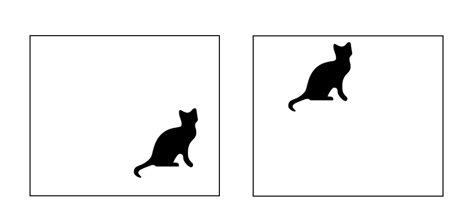
Трансляционная симметрия: Тот же объект в различных местах.

Для нас, людей, не важно, если кошка в правом нижнем углу или где-то в верху картинки. В обоих случаях мы найдем кошку. Мы можмем сказать, что наш человеческий детектор котов трансляционно инвариантен.

Однако, если мы посмотрим на архитектуру типичной полносвязанной сети, мы можем понять, что нет ничего, что на самом деле может предостеречь эту сеть работать верно только в какой-то части картинки. Вопрос который мы задаем: Есть ли способ сделать нейронную сеть трансляционно инвариантной?

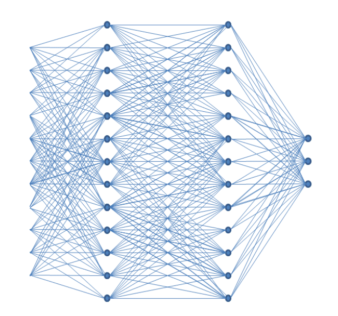
Полносвязанная нейронная сеть с двумя скрытыми слоями.

Давайте взглянем ближе на картинку кошки. Скоро мы поймем, что пиксели отражающие котячую голову более связанны, чем другие пиксели связанные с кошачим хвтостом. Отсюда, мы так же можем захотеть сделать нашу нейронную сеть такой редкой, что нейроны в следующем слое будут связаны только с соотвествующими соседними пикселями. Таким образом, каждый нейрон в следующем слое будут отвечать только за маленькие свойства оригинальной картинки. Участок который видит нейрон назовем полем восприятия.

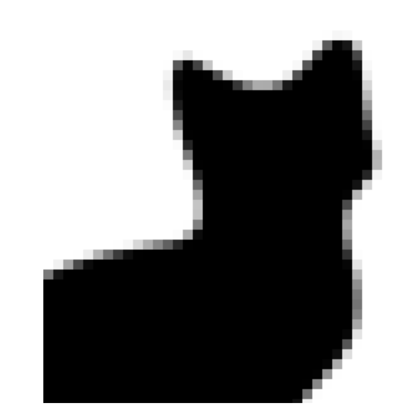
Соседние пиксели дают более связную информацию чем отдаленные. Увеличим картинку кошки.

Сверточная нейронная сеть CNN или просто ConvNets была спроектированна для решения двух проблем: трансляционная симметрия и положение изображения. Первое, давайте определим понятие свёрточный оператор.

Возможно вы не знаете, но очень похоже вы уже встречали сверточные фильтры. Вспомните когда вы впервые играли с графическим редактором типа GIMP или Photoshop. Возможно вы были восхищены возможностью эффектов таких как корректировка четкости, замыливание или определение краёв. Если нет, тогда вы должны это попробовать. Секрет этих фильтров в том, что это сверточное применение ядра картинки. Ядро картинки это матрица 3x3, как представленно ниже.

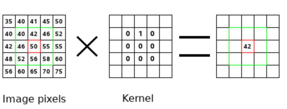
Простой сверточный шаг: Не путайте значение пикселя и ядро.

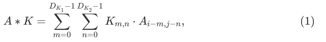
Ниже представлен простой сверточный шаг. Этот шаг - скалярное произведение ядра и значений пикселей. Так как все значения ядер исключая вторые единицы в первом нуле, то результат равняется второму значению в первой строке зеленой рамки. т.о. 40⋅0+42⋅1+46⋅0+…+58⋅0=42. Сверточный оператор берет картинку и действует внутри зеленого перемещающегося окна для того чтобы произвести скалярное произвдение всех частей картинки. Результат новая отфильтрованная картинка. 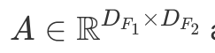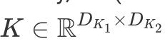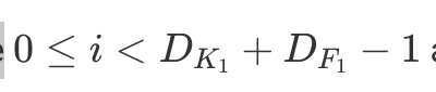Метематически, прямой сверточный оператор (*) между картинкой and a kernel можно выразить следующим образом где and 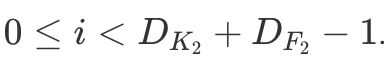Для лучшего понимания что происходит, можно поиграться с другой картинкой.

В чем идея применения оператора двигающегося окна или свертки? В основании идеи лежит биология. Человеческий глаз имеет ограниченное поле четкого зрения. Мы воспринимаем объекты в целом постоянно передвигая взгляд по объекту. Эти быстрые движения называются саккады. Отсюда, сверточный оператор может быть описан как простая модель естественное восприятие объекта глазом. Важный момент, что свертка достигает постоянство сдвига благодаря методу движемого окна. Даже больше, так как каждый результат связан через ядро с очень ограниченным числом пикселей в начальном изображении, сверточная связь очень редки. Поэтому, используя свертки в нейронных сетях мы достигаем инвариантность и разреженость связей. Давайте посмотрим, как это работает на практике.

Архитектура сверточной нейронной сети.

Интересное своейтсво сверточного слоя заключается в том, что если мы подаем на вход смещенную картинку, то выходная карта будет свдинута на ту же величину, в противно случае оно останется неизменным. Это свойство является базовым в надежности сверточной сети при сдвиге или искажении вводных данных.

Как только свойство было замечено, его точно место положение становится не важным. А важным становится, только примерная относительная позиция.

Lecun et al. Gradient-based learning applied to document recognition (1998)

Прототип того, что сегодня мы называем сверточной нейронной сетью была предложена в 1970 году Фукусимой. Было предложено можество методов обучения с учителем и без, но сегодня CNN обучается только благодаря обратному распространению. Давайте взглянем на одну из известных архитектур известных как LeNet-5.

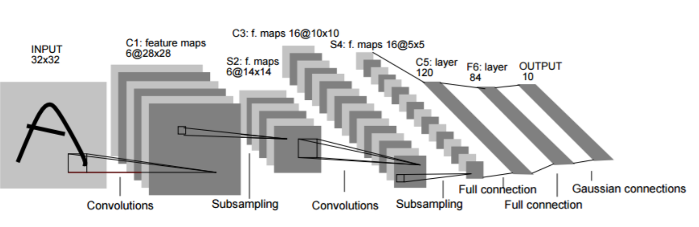
LeNet-5 architecture from Lecun et al. Gradient-based learning applied to document recognition.

Архитектура очень близка к современным CNN. LeNet-5 был создан для распознавания ручных цифр с чернобелых картинок размером 32x32. Два основных блока, как мы сейчас их называем: экстрактор и классификатор свойств.

С локальными восприимчивыми полянми нейронов можно извлечь простые визуальные свойства, как ориентация граней, концы, углы...

Lecun et al. Gradient-based learning applied to document recognition (1998)

Экстрактор свойств состоит из двух сверточных слоёв. Первый слой имеет 6 сверточных фильтров с ядром 5x5. Применение этих фильтров с подпоследовательными добавочными смещениями и гиперболической танценциальной активацией производят карты, естественно новые, чуть меньшего размера 28x28. По соглашению, результат описывается следующим объёмом 28x28x6. Чтобы сократить разреженное разрешени, производится подрезание. Оно выдает карты свойств 14x14x6.

Все юниты в карте свойств делят тот же набор 25 весов и тем же количеством смещений, так чтобы можно было заметить те же свойства в любом месте на входе. Lecun et al. Gradient-based learning applied to document recognition (1998)

Следующая свертка округляет результат уже в размер карт 10x10x16. В отичии от первого слоя, мы используем ядро 5x5x6. Это значит, что каждый из 16 сверток одновременно обрабатывает все 6 свойств карты полученных на прошлом шаге. После разделения мы получаем результирующи размер 5x5x16.

Классификатор состоит из трехмерно связанных слоёв с 120, 84б и 10 нейронами каждый. Последний слой предоставляет зашифрованный ответ. Небольшое различие между современными архитектурами в последнем слое, который состоит из 10 эвклидовых радиальных смещеных функциональных единиц, где сегодня это будет обычный полносвязный слой следующим за слоем softmax.

Важно понять, что единичный сверточный фильтр может понять только одно свйоство. Например, он может понять горизонатальную линию. Поэтому мы используем несколько больше фильтров с различными ядрами, чтобы иметь возможность понимать свойства: вертикальные линии, простые текстуры, или углы. Как вы уже видели, число фильтров обычно отображается в ConvNet диаграмма как объем. Слои, что глубже в сети будут объединять базовые свойства что были найдены в слоях выше в более абстрактные сущности как глаз, ухо или даже полные фигуры. Чтобы лучше понять этот механизм, давайте мы взглянем на поле восприятия на визуализации ниже.

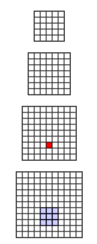
Поле графического восприятия унаследованно от Арун Маллуа. Проведем курсором мыши над любым нейроном в верхнем слое, чтобы посмотреть как расширится поле восприятия в слое дальше.

Как можно увидеть проверяя нейроны в последнем слое, даже маленькое поле 3x3 ратстет как происходит движение в первом слое. Мы можем предвидеть, что нейроны "глубже" будут иметь лучшее понимание, что происходит на картинке.

Красота и величие достигаемое глубоким обучением в том, что ядро фитрации самообучаемо самой сетью, достигается оно даже лучшую точность в сравнении с человеческими способностями. Странности сверточных слоев в том, что результат получаемые после повторяющихся применений маленького количества веса как определено в ядре. Благодаря весам, сверточные слои имеют резко сокращенное число обучаемых параметров, сравнимых с полносвязанными слоями.

Сверточные типы

Я решил включить эту часть для интересующихся. Если вы впервые встретились с CNN, можете пропустить эту часть и вернуться к ней позже.

Можно встрерить большое количество слухов вокруг сверточных сетей сегодня. Однако, это не делает яснее, что те слои компьютерного зрения, что опускаются ниже, часто отличаются от тех, что исследуются для ConvNet. Даже в ConvNet есть множество сверточных слоев воодушевлящих зарождение ConvNet архитектуры и окруженных Xception и Mobilenet работами. Я верю, что вы заслуживаете знать, что существует множество видов применения сверточной сети в разных контекстах и я должен вам подсказать путь.

Свертка компьютерного зрения

Низкоуровневое компьютерное зрение, например графические редакторы, обычно работают с одним, тремя, четырмя каналами картинки(красный, зеленый, синий, прозрачность). Каждое отдельное ядро обычно применяется на каждый канал. В этом случае получаем столько каналов, сколько каналов на входном изображении. В редких случаях когда одно ядро применяется к каждому каналу(размытие). Иногда, результирующие каналы суммируются производя одноканальную картинку(определение границ).

Свертка похожая на LeNet

Чистая свертка CV отличается от этих ConvNet по 2м причинам: CV ядра определяются в ручную, где сила нейронной сети идет от обучения, и в нейронной сети мы строим глубокую сткруктуру составляя множество сверток друг на друга. Отсюда, нам нужно пересобрать информацию идущую от прошлого слоя. Оно позволяет нам обучать высший уровень понимания свойств. На конец свертки в нейронных сетях могут содежрать определения смещения, т.е. константы добавленые в результате работы каждой свертки.

A pure CV-style convolution is different from those in ConvNets due to two reasons: (1) in CV kernels are manually defined, whereas the power of neural networks comes from training, and (2) in neural networks we build a deep structure by stacking multiple convolutions on top of each other. Therefore, we need to recombine the information coming from previous layers. That allows us to train higher-level feature detections8. Finally, convolutions in neural networks may contain bias terms, i.e. constants added to results of each convolution.

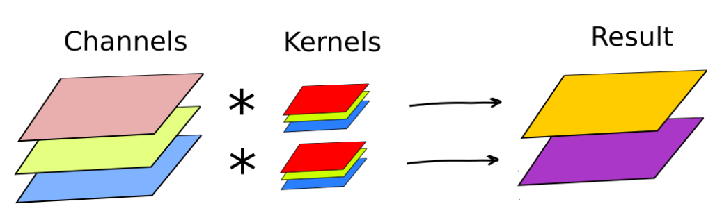
Recombination of features coming from earlier layers was previously illustrated in LeNet-5 example. As you remember, in the second convolutional layer we would apply 3D kernels of size 5×5×6 computing dot products simultaneously on all six feature maps from the first layer. There were sixteen different kernels thus producing sixteen new channels.

Each pixel in the feature map is obtained as a dot product between the RGB color channels and the sliding kernel. Image credit: Wikimedia. Convolution filter with three input channels. Each pixel in the feature map is obtained as a dot product between the RGB color channels and the sliding kernel. Image credit: Wikimedia.

To summarize, a single LeNet-like convolution operates simultaneously on all input channels and produces a single channel. By having an arbitrary number of kernels, any number of output channels is obtained. It is not uncommon to operate on volumes of 512 channels! The computation cost of such convolution is DK×DK×M×N×DF×DF where M is the number of input channels, N is the number of output channels, is the kernel size and is the feature map size9.

Depthwise Separable Convolution

LeNet-style convolution requires a large number of operations. But do we really need all of them? For instance, can spatial and cross-channel correlations be somehow decoupled? The Xception paper largely inspired by Inception architecture shows that indeed, one can build more efficient convolutions by assuming that spatial correlations and cross-channel correlations can be mapped independently. This principle was also applied in Mobilenet architectures.

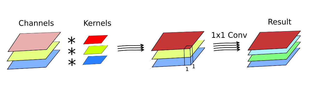
The depthwise separable convolution works the following way. First, like in low-level computer vision, individual kernels are applied to each individual channel. Then, after optional activation10, there is another convolution, but this time exclusively in-between channels. That is typically achieved by applying a 1×1 convolution kernel. Finally, there is a (ReLU) activation.

This way, depthwise separable convolution has two distinct steps: a space-only convolution and a channel recombination. This reduces the number of operations to

To summarize, the main difference between low-level image processing (Photoshop) and neural networks is that image processing operates on lots of pixels, but the image depth remains unchanged (three-four channels). On the other hand, convolutional neural networks tend to operate on images of moderate width and height (e.g. 230×230 pixels), but can achieve depth of thousands of channels, while simultaneously decreasing the number of "pixels" in feature maps towards to the end of processing pipeline.

Implementing Convolutional Networks in Haskell

Today, we will implement and train a convolutional network inspired by LeNet-5. We will witness that indeed this ConvNet has about twice lower error on the MNIST handwritten digit recognition task, while being four times smaller compared to the previous model! The source code from this post is available on Github.

Convolutional Layer Gradients

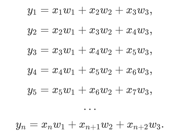
First of all, we need to know how to obtain convolutional layer gradients. Although convolution in neural networks is technically performed by the cross-correlation operator11, this does not matter since kernel parameters are learnable. To understand gradient derivation, let us take a look at the cross-correlation operation in single dimension:

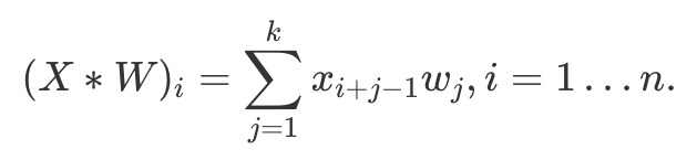
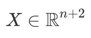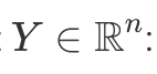
For instance, if we fix 1D kernel W size to be k=3, equation above would simply mean that vector produces an output Denoting error from the previous layer as δ, convolutional layer gradients w.r.t. input X are

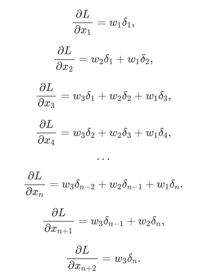
So it can be seen that it is a cross-correlation operation again, but with flipped kernel. Hence

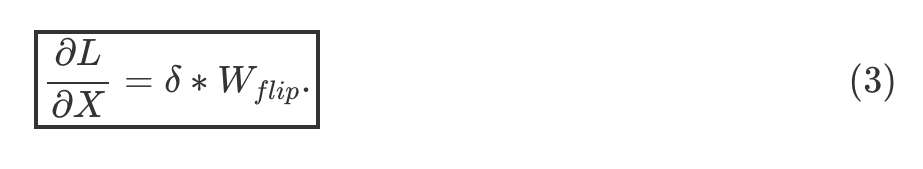
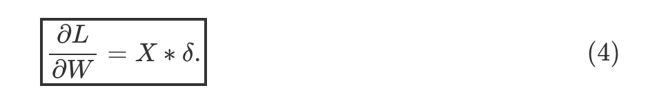
Similarly, gradients w.r.t. kernel W are computed as Thus we have yet another cross-correlation

These formulas will become handy when implementing the backward pass from convolutional layers.

Convolutions in Haskell

First, let us start with two most relevant imports: modules from array library massiv and automatic differentiation tools from backprop.

-- Multidimensional arrays to store learnable
-- parameters and represent image data
import           Data.Massiv.Array hiding ( map, zip, zipWith, flatten )
import qualified Data.Massiv.Array as A
-- Automatic heterogeneous back-propagation library
import           Numeric.Backprop

Let us brush up our data structures to match our convolutional needs. First, we need to represent a batch of images. We will use the following convention: batch size × channels × height × width. For instance, if we have a batch of 16 RGB images with dimensions 32 × 32 , then we get a volume of 16 × 3 × 32 × 32. Here we have a Volume4 type:

type Volume4 a = Array U Ix4 a

It is just an alias to a four-dimensional unboxed Array coming from the massiv package. In deep learning frameworks those n-dimensional arrays are conventionally called tensors. Note that during transformation in a neural network, the shape of data will change, except the batch dimension that will always remain the same. Similarly, we need a way to represent our convolutional filters. In LeNet, for instance, we can represent the first convolutional layer as a volume of 6×1×5×5. In order to be able to distinguish between parameter and data volumes, we will introduce Conv2d data structure:

data Conv2d a = Conv2d { _kernels :: !(Volume4 a) }

Note that for the sake of simplicity we decided not to implement biases. As previously, Linear will represent fully-connected layer parameters:

data Linear a = Linear { _weights :: !(Matrix a)
                       , _biases :: !(Vector a)
                       }

As usual, type parameter a means that we may later decide whether we need a Float, a Double or some other weights encoding. Now, we have everything to describe learnable parameters (weights) in LeNet:

data LeNet a =
    LeNet { _conv1 :: !(Conv2d a)
          , _conv2 :: !(Conv2d a)
          , _fc1 :: !(Linear a)
          , _fc2 :: !(Linear a)
          , _fc3 :: !(Linear a)
          }

Now, it becomes obvious that with every new layer type managing backpropagation data structures as we did on Days 2 and 4 quickly becomes tedious. Moreover, last time when we introduced a Batchnorm1d layer, our forward-backward pass function already oversized 100 lines of code. Today, we will make use of the backprop library introduced on Day 3 to better structure our project. Thus, LeNet can be represented as a differentiable function lenet, which is nothing more than a composition of other functions aka neural network layers:

lenet :: (Reifies s W)
      => BVar s (LeNet Float)
      -> Volume4 Float  -- ^ Batch of images
      -> BVar s (Matrix Float)
lenet l = constVar

          -- Feature extractor
          -- Layer (layer group) #1
          ~> sameConv2d (l ^^. conv1)
          ~> relu
          ~> maxpool
          -- Layer #2
          ~> validConv2d (l ^^. conv2)
          ~> relu
          ~> maxpool

          ~> flatten

          -- Classifier
          -- Layer #3
          ~> linear (l ^^. fc1)
          ~> relu
          -- Layer #4
          ~> linear (l ^^. fc2)
          ~> relu
          -- Layer #5
          ~> linear (l ^^. fc3)

This description pretty much talks for itself. The (~>) operator is a function composition, i.e. f ~> g = \x -> g(f(x)). This could be written in other forms, though. We prefer the so-called pointfree notation:

(~>) :: (a -> b) -> (b -> c) -> a -> c
f ~> g = g. f

That simply reverses the order of composition, i.e. first is applied f, and only then g12. I find this "backward composition" notation consistent with major neural network frameworks. Compare how an equivalent network can be represented in PyTorch:

import torch.nn as nn

class LeNet(nn.Module):
    def __init__(self, num_classes=10):
        super(LeNet, self).__init__()
        # Feature extractor: a (sequential) composition of convolutional,
        # activation, and pooling layers
        self.features = nn.Sequential(
            nn.Conv2d(1, 6, kernel_size=5, stride=1, padding=2, bias=False),
            nn.ReLU(),
            nn.MaxPool2d(kernel_size=2, stride=2),
            nn.Conv2d(6, 16, kernel_size=5, stride=1, padding=0, bias=False),
            nn.ReLU(),
            nn.MaxPool2d(kernel_size=2, stride=2)
        )

        # Classifier: a composition of linear and activation layers
        self.classifier = nn.Sequential(
            nn.Linear(16 * 5 * 5, 120, bias=True),
            nn.ReLU(),
            nn.Linear(120, 84, bias=True),
            nn.ReLU(),
            nn.Linear(84, num_classes, bias=True)
        )

    # Composition of feature extractor and classifier
    def forward(self, x):
        x = self.features(x)
        # Flatten
        x = x.view(x.size(0), -1)
        x = self.classifier(x)
        return x

Despite some noise in the Python code above13, we see that nn.Sequential object acts simply as a function composition with (~>) combinators. Now, let us return back to lenet signature:

lenet :: (Reifies s W)
      => BVar s (LeNet Float)
      -> Volume4 Float  -- ^ Batch of images
      -> BVar s (Matrix Float)

We have already seen the BVar s ("backprop variable") type meaning that we deal with a differentiable structure. The first argument has type BVar s (LeNet Float). That conventionally means that LeNet is the model optimized by backpropagation and shortly we will show how to achieve that. The second function argument is a batch of images (Volume4), and finally the result is a bunch of vectors (Matrix) containing classification results performed by our model.

Functions constVar and (^^.) are special ones. Both are coming from the Numeric.Backprop import. The first function "lifts" a batch to be consumed by the sequence of differentiable functions. The second one (^^.) allows us to conveniently access records from our LeNet data type. For instance, sameConv2d (l ^^. conv1) means that sameConv2d has access to the _conv1 field.

Layers known from the previous days (linear, ReLU) will be reused in accordance to backprop conventions. What is left to implement are sameConv2d, validConv2d, and maxpool layers. To be able to do that simply and efficiently we will learn a neat tool called stencils.

Fun With Stencils

Let us come back to 1D convolution from Equation (2). If we look closer, we notice a pattern in convolution/cross-correlation, i.e. 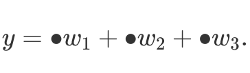Indeed, every time we multiply the same set of weights and the only thing that changes is source data (masked with bullets above). Therefore, to implement convolutions we only need to define some sort of pattern that processes given points. This fixed pattern applied to array elements is called a stencil. The stencil convolution approach can be also used to perform subsampling operations, e.g. max pooling. Moreover, the method allows for efficient data parallelism.

Previously, we have introduced Massiv library featuring parallel arrays computation. This library was preferable to hmatrix due to two reasons: multidimensional arrays and parallel computation. Today, we have yet one more reason: stencils. Good news: massiv already implements them for us! Those are based on this work.

First, we warm up with a 1D cross-correlation from Equation (2). Suppose, we have a "delay" kernel [1,0,0]. Here is how this can be applied in an interactive shell (aka REPL):

> import Data.Massiv.Array
> type Vector a = Array U Ix1 a  -- Convenience alias
> k = fromList Par [1, 0, 0] :: Vector Int
> sten = makeCorrelationStencilFromKernel k
> dta = fromList Par [1, 2, 5, 6, 2, -1, 3, -2] :: Vector Int
> mapStencil (Fill 0) sten dta
Array DW Par (Sz1 8)
  [ 0, 1, 2, 5, 6, 2, -1, 3 ]

Note that the first value was replaced with zero since we have applied mapStencil (Fill 0) that uses zero-filling padding strategy to preserve the size of the array. Our array was processed to look internally like this: [0,1,2,5,6,2,−1,3,−2,0], with fake zeros inserted. Alternatively, we could use applyStencil noPadding as below:

> applyStencil noPadding sten dta
Array DW Par (Sz1 6)
  [ 1, 2, 5, 6, 2, -1 ]

> dta' = fromList Par [0, 1, 2, 5, 6, 2, -1, 3, -2, 0] :: Vector Int
> applyStencil noPadding sten dta'
Array DW Par (Sz1 8)
  [ 0, 1, 2, 5, 6, 2, -1, 3 ]

Here is a more interesting computer vision example. For comparison, we define an identity (no transformation) stencil and a box stencil (blurring effect). The identity kernel has one in its center (coordinate 0 :. 0) and zeroes everywhere else. The box transformation computes averaged value over nine neighboring pixels including the center pixel itself (see also this for more information), therefore the kernel has weights 1/9 everywhere.

import Data.Massiv.Array
import Data.Massiv.Array.IO
import Graphics.ColorSpace

identity :: Elevator a => Stencil Ix2 (Pixel RGB a) (Pixel RGB a)
identity =
  makeStencil sz c $ \get -> get (0 :. 0)
  -- `get` is a function that receives a coordinate relative to the
  -- stencil's center, i.e. (0 :. 0) is the center itself.
  where
    sz = Sz (3 :. 3)  -- Kernel size: 3 x 3
    c = 1 :. 1  -- Center coordinate
{-# INLINE identity #-}

box :: (Elevator a, Fractional a) => Stencil Ix2 (Pixel RGB a) (Pixel RGB a)
box =
  makeStencil sz c $ \get ->
    ( get  (-1 :. -1) + get  (-1 :. 0) + get (-1 :. 1)
    + get  (0 :. -1) + get  (0 :. 0) + get (0 :. 1)
    + get  (1 :. -1) + get  (1 :. 0) + get (1 :. 1)) / 9
  where
    sz = Sz (3 :. 3)
    c = 1 :. 1
{-# INLINE box #-}

main :: IO ()
main = do
  frog <- readImageAuto "files/frog.jpg" :: IO (Image S RGB Double)

  -- Identity transformation
  writeImageAuto "files/frog_clone.png" $ computeAs S (mapStencil Edge identity frog)
  -- Box filtering (blur)
  writeImageAuto "files/frog_blurred.png" $ computeAs S (mapStencil Edge box frog)

In main function, we load an image and apply those two stencils. All we need to do is to specify the stencil pattern, i.e. convolution kernel, and massiv takes care to apply it. This is what we get:

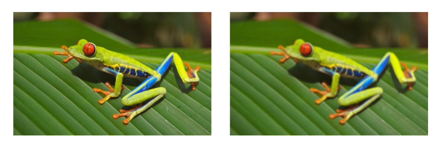
Original frog (left) and blurred (right). Image credit. While in the last example above we have defined stencils manually with makeStencil, in practice we may prefer to use

makeCorrelationStencilFromKernel
  :: (Manifest r ix e, Num e) => Array r ix e -> Stencil ix e e

The function has a single argument, stencil's kernel.

Convolutional Layers With Stencils

Before actually diving into implementation, we have to understand that convolution decreases the number of "pixels" in the image, similar to the "delayed" 1D kernel above. Moreover, some information next to the image border is lost due to the fact that the sliding window "visits" bordering pixels less than those closer to the center. To avoid the information loss, often the area around the image is "padded" (filled) with zeros. Thus we can perform a "same" convolution, i.e. one that does not change the convolved dimensions. As of version 0.4.3, Massiv stencils already support different padding modes. In case of LeNet 5×5 kernels, we define padding of 2 pixels on every side (top, right, bottom, and left) using top left and bottom right corners:

sameConv2d = conv2d (Padding (Sz2 2 2) (Sz2 2 2) (Fill 0.0))

"Valid" convolution is a convolution with no padding:

validConv2d = conv2d (Padding (Sz2 0 0) (Sz2 0 0) (Fill 0.0))

In both cases, we will use generic conv2d function with a padding argument. Supporting automatic differentiation, our conv2d combines both forward and backward passes:

conv2d :: Reifies s W
       => Padding Ix2 Float
       -> BVar s (Conv2d Float)
       -> BVar s (Volume4 Float)
       -> BVar s (Volume4 Float)

The signature tells us that it is a differential function that takes a padding, Conv2d parameters, and a batch of images Volume4 and produces another batch of images. The most efficient way to define the function is to manually specify both forward and backward passes; although it is also possible to specify only the forward pass composing smaller functions operating on BVars and letting backprop to figure out their gradients. The general pattern in backprop is to provide the forward pass (Conv2d w) x -> ... and the backward pass using a lambda expression containing previously computed gradients dz as an argument. Those forward and backward passes are glued together with liftOp2. op2 (or liftOp1. op1 for layers with no learnable parameters) as below:

conv2d p = liftOp2. op2 $ \(Conv2d w) x ->
  (conv2d_ p w x, \dz -> let dw = conv2d'' p x dz
                             -- ... Compute padding p1
                             dx = conv2d' p1 w dz
                         in (Conv2d dw, dx) )

Now, forward pass is a cross-correlation between the input channels and a kernel set from the filter bank. Recall that the number of kernel sets defines the number of output channels. We simultaneously perform cross-correlation operations on all images in the batch, therefore we concatenate the results over the channel dimension 3.

conv2d_ pad w x = res
  where
    -- Some code omitted for simplicity

    -- Create a stencil ("sliding window") from the given set
    -- in the filter bank
    sten = makeCorrelationStencilFromKernel. resize' (Sz4 1 cin w1 w2). (w !>)

    -- For each kernel set, create and run stencils on all images in the batch.
    -- Finally, concatenate (append) the results over the channel dimension
    res = foldl' (\prev ch -> let conv = computeAs U $ applyStencil pad4 (sten ch) x
                              in computeAs U $ append' 3 prev conv) empty [0..cout - 1]

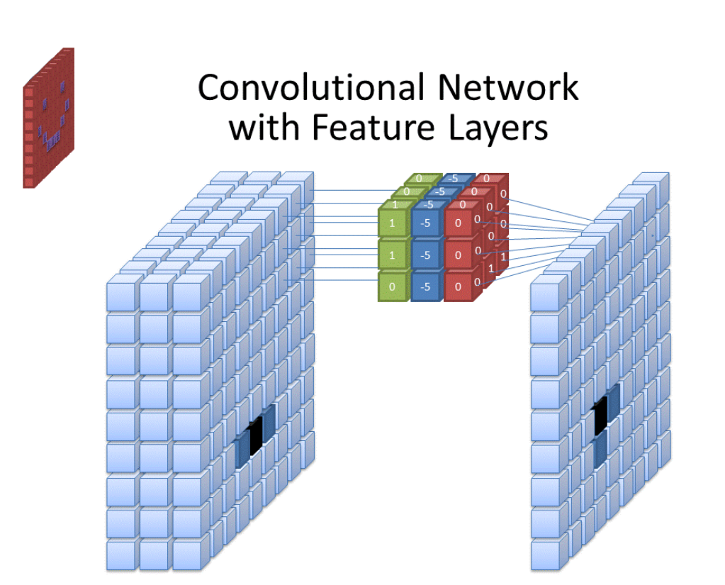
To better illustrate how this works on a batch of images, here is a visualization what is going on in the first convolutional layer.

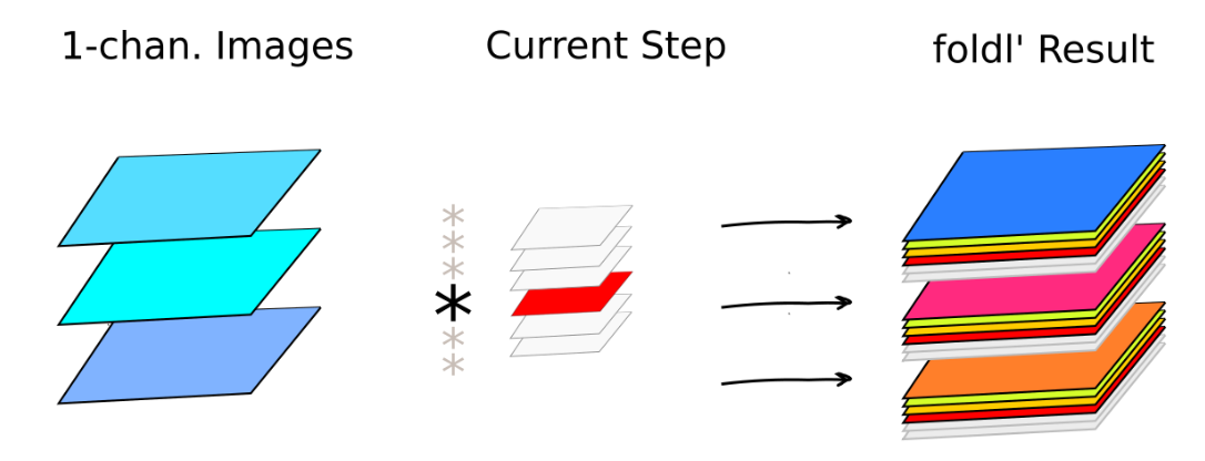
Folding over six filter sets in the first convolutional layer. Currently active convolutional filter set (highlighted in red) contributes to so far processed results (in color) on the right. Folding over six filter sets in the first convolutional layer. Currently active convolutional filter set (highlighted in red) contributes to so far processed results (in color) on the right.

In MNIST we have black and white images, thus a single-channel input. During each step in foldl', a single filter is applied to all images. There are six filters hence resulting in six new channels in each convolved image on the right. A similar operation is performed in the second convolutional layer, this time resulting in 16-channel images (see also Convolution Types. LeNet-like Convolution above for the illustration on a single image). Below is a Python/NumPy equivalent of foldl'/applyStencil combo from above.

import numpy as np

# ... Get current batch, stride, and padding parameters
# ... Using those parameters, determine
# output image width, height, and number of channels

# Initialize resulting array
res = np.zeros([len(batch), out_channels, out_im_height, out_im_width])

# Iterate over all four dimensions
for i in range(len(batch)):
    for j in range(out_im_height):
        for k in range(out_im_width):
            for c in range(out_channels):
                # Define the sliding window position
                y1 = j * stride
                y2 = y1 + kernel_height
                x1 = k * stride
                x2 = x1 + kernel_width
                im_slice = batch[i, :, y1:y2, x1:x2]

                # Get current channel weights
                Wcur = W[:,c,:,:]

                # Out pixel = dot product
                res[i, c, j, k] = np.sum(im_slice * Wcur)

return res

Now that we have accomplished convolution in the forward direction, we need to compute gradients for the backward pass.

Gradients Are Also Convolutions

The image plane gradients are obtained by formulas (3) and (4). However, in practice we also have to take into account that we deal with multiple images that have multiple channels. In fact, I leave it to you to figure out exact formulas. Those can be inferred from Haskell equations below. Yes, any Haskell line is already written in a mathematical notation. That is essentially what Haskell "purity" is about. You might have realized by now that programming in Haskell is all about finding your own patterns. Now, let us compute gradients w.r.t. input

conv2d' p w dz = conv2d_ p w' dz
  where
    w' = (compute. rot180. transposeInner) w

    -- Rotate kernels by 180 degrees. This is expressed in terms
    -- of tensor reversal along width and height dimensions.
    rot180 = reverse' 1. reverse' 2

Let us remind that these compute functions evaluate delayed arrays into actual representation in memory. Please do not hesitate to find reverse and transposeInner in massiv documentation. Finally, here we have gradients w.r.t. convolution kernel weights

conv2d''
  :: Padding Ix2 Float -> Volume4 Float -> Volume4 Float -> Volume4 Float
-- Iterate over images in a batch
conv2d'' p x dz = res  -- computeMap (/fromIntegral bs) res
  where
    -- Batch size
    Sz (bs :> _) = size x

    -- Code omitted

    res = foldl' (\acc im ->
      let cur = _conv2d'' p (compute $ dzd !> im) (compute $ xd !> im)
       in acc + cur) base [1..bs-1]

We simply accumulate gradients from individual images in the batch using left strict fold. Finally, we generalize Equation (4) to get those transformations:

_conv2d'' :: Padding Ix2 Float
          -> Volume Float  -- ^ Gradients \delta (dz)
          -> Volume Float  -- ^ X
          -> Volume4 Float  -- ^ dL/dW
_conv2d'' (Padding (Sz szp1) (Sz szp2) pb) dz x = ...

More Stencils: Max Pooling Layers

Stencils are handy not only for convolutional layers. Another use case are pooling (subsampling) layers. To be able to perform max pooling, first we have to define the corresponding stencil pattern (or just use maxStencil from the library instead).

maxpoolStencil2x2 :: Stencil Ix4 Float Float
maxpoolStencil2x2 = makeStencil (Sz4 1 1 2 2) 0 $ \ get ->
  let max4 x1 x2 x3 x4 = max (max (max x1 x2) x3) x4
   in max4 <$> get (0 :> 0 :> 0 :. 0)
           <*> get (0 :> 0 :> 1 :. 1)
           <*> get (0 :> 0 :> 0 :. 1)
           <*> get (0 :> 0 :> 1 :. 0)

Here max4 is a function that receives four values and computes the maximal one. This function is applied to a patch of four neighboring pixels. Do not forget that we operate in a 4D space, therefore each point in the given patch has four coordinates. Here is how we interpret a coordinate:

 (0 :> 0 :> 0 :. 0)
  ^    ^    ^    ^
  4    |    |    1
       3    2
1 and 2 are coordinates in the image plane,
3 is the channel dimension, and
4 is the batch dimension.

Note the :. and :> operators. The first one :. constructs a coordinates (index) "list" with two elements and :> just adds more coordinates for higher dimensions. To learn more about <$> and <*> functions, see Applicative Functors.

We would like to have non-overlapping sliding windows in max pooling, therefore, we want to use 2×2 stride in the image plane. However, we would like to perform the same operation over every channel in every image. Therefore, we use computeWithStride and the stride is 1 :> 1 :> 2 :. 2 (batch dim×channel dim×height×width). Note that we do not want any padding since the goal of pooling is actually to reduce the number of pixels: four times in this case.

maxpool_ :: Volume4 Float -> Volume4 Float
maxpool_ = computeWithStride (Stride (1 :> 1 :> 2 :. 2)).
             applyStencil noPadding maxpoolStencil2x2

Finally, we compute gradients using pixels that had maximal values in the forward pass. And we obtain a differentiable maxpool function lifting forward-backward passes with liftOp1. op1:

maxpool :: Reifies s W
        => BVar s (Volume4 Float)
        -> BVar s (Volume4 Float)
maxpool = liftOp1. op1 $ \x ->
  let out = maxpool_ x
      s = Stride (1 :> 1 :> 2 :. 2)
      outUp = computeAs U $ zoom s out
      maxima = A.zipWith (\a b -> if a == b then 1 else 0) outUp x
  in (out, \dz -> let dzUp = computeAs U $ zoom s dz
                  -- Elementwise product
                  in maybe (error $ "Dimensions problem") compute (maxima .*. delay dzUp))

Putting It All Together

First, we fetch the MNIST data and randomly generate the initial model:

main :: IO ()
main = do
  trainS <- mnistStream 64 "data/train-images-idx3-ubyte" "data/train-labels-idx1-ubyte"
  testS <- mnistStream 1000 "data/t10k-images-idx3-ubyte" "data/t10k-labels-idx1-ubyte"

  net <- randNetwork

As previously, data streams are loaded from binary MNIST files; however, the initial model generation has to take into account the new structure, LeNet.

randNetwork :: IO (LeNet Float)
randNetwork = do
  -- Generate a new conv layer weights:
  -- 6 out channels, 1 input channel, kernel size: 5 x 5
  _conv1 <- randConv2d (Sz4 6 1 5 5)
  -- 16 out channels, 6 input channels, kernel size: 5 x 5
  _conv2 <- randConv2d (Sz4 16 6 5 5)
  let [i, h1, h2, o] = [16 * 5 * 5, 120, 84, 10]
  _fc1 <- randLinear (Sz2 i h1)
  _fc2 <- randLinear (Sz2 h1 h2)
  _fc3 <- randLinear (Sz2 h2 o)
  return $
    LeNet { _conv1 = _conv1
          , _conv2 = _conv2
          , _fc1 = _fc1
          , _fc2 = _fc2
          , _fc3 = _fc3
          }

Finally, we train our model

  -- ... `main` function
  net' <- train TrainSettings { _printEpochs = 1
                              , _lr = 0.01
                              , _totalEpochs = 30
                              } net (trainS, testS)

The train function is essentially a wraper around the sgd stochastic gradient descent function.

train TrainSettings { _printEpochs = printEpochs
                    , _lr = lr
                    , _totalEpochs = totalEpochs
                    } net (trainS, testS) = do
  (net', _) <- iterN (totalEpochs `div` printEpochs) (\(net0, j) -> do
    net1 <- sgd lr printEpochs net0 trainS

    -- ... Compute and print accuracies

    ) (net, 1)
  return net'

In sgd we compute gradients over a mini-batch and subtract them to optimize the model parameters.

sgd lr n net0 dataStream = iterN n epochStep net0
  where
    -- Fold over the stream of all batches
    epochStep net = S.foldl' _trainStep net dataStream
    -- Update gradients based on a single batch
    _trainStep net (x, targ) = trainStep lr x targ net

Now, the training step is a few lines of code thanks to Numeric.Backprop.gradBP function that applies the chain rule, thus replacing the entire pass function we had before.

trainStep
  :: Float  -- ^ Learning rate
  -> Volume4 Float  -- ^ Images batch
  -> Matrix Float  -- ^ Targets
  -> LeNet Float  -- ^ Initial network
  -> LeNet Float
trainStep lr !x !targ !n = n - lr * (gradBP (crossEntropyLoss x targ) n)

If we ever want to actually use our model to identify a handwritten digit, we call evalBP:

forward :: LeNet Float -> Volume4 Float -> Matrix Float
forward net dta = evalBP (`lenet` dta) net

Now, we compile and run our program:

$ ./run.sh
1 Training accuracy 10.4  Validation accuracy 10.3
2 Training accuracy 85.7  Validation accuracy 86.3
3 Training accuracy 95.9  Validation accuracy 96.2
4 Training accuracy 97.6  Validation accuracy 97.4
5 Training accuracy 98.4  Validation accuracy 98.1
6 Training accuracy 98.3  Validation accuracy 98.0
7 Training accuracy 99.0  Validation accuracy 98.8
8 Training accuracy 99.0  Validation accuracy 98.7
9 Training accuracy 99.1  Validation accuracy 98.7
...
26 Training accuracy 99.8  Validation accuracy 99.0
27 Training accuracy 99.8  Validation accuracy 98.7
28 Training accuracy 99.9  Validation accuracy 98.9
29 Training accuracy 99.7  Validation accuracy 98.6
30 Training accuracy 99.9  Validation accuracy 98.9

Thus, after 30 training epochs, we have obtained a ∼1% validation error, which is about twice as low compared to the simple fully-connected architecture. See the complete project on Github.

Model Parameters Comparison

Our three-layer model from Day 4 consumed (784+1)⋅300+(300+1)⋅50+(50+1)⋅10=251,060 learnable parameters (not counting batchnorm parameters). In contrast, the convolutional neural network model that we have implemented today requires only 1 ⋅5⋅5⋅6+16⋅6⋅5⋅5+(400+1)⋅120+(120+1)⋅84++(84+1)⋅10=61,684 parameters. Note also that 1⋅5⋅5⋅6+16⋅6⋅5⋅5=2,550 are convolutional layers parameters, whereas the majority (59,134) reside in classifier's fully-connected layers.

Although, we did not apply batch normalization today, like was in the original LeNet, feel free to experiment with adding batchnorm layers. Please also note that there is a difference between batch normalization after convolution and after fully-connected layers (see the batchnorm article).

Citation

@article{penkovsky2019CNN,
 title   = "Convolutional Neural Networks Tutorial",
 author  = "Penkovsky, Bogdan",
 journal = "penkovsky.com",
 year    = "2019",
 month   = "November",
 url     = "https://penkovsky.com/neural-networks/day5/"
}

Summary

Convolutional neural networks aka ConvNets achieve translation invariance and connection sparsity. Thanks to weight sharing, ConvNets dramatically reduce the number of trained parameters. The power of ConvNet comes from training convolution filters, in contrast to manual feature engineering. In future posts, we will gain the power of GPU to face bigger challenges. We will save the planet. And we might even try to read someone's mind with convolutional networks. Stay tuned!