День 5: Сверточные нейронные сети
Сегодня мы поговорим об одной из самых важных архитектур глубокого обучения, так сказать алгоритм всех алгоритвом в компьютерном зрении. Today we will talk about one of the most important deep learning architectures, the "master algorithm" in computer vision. That is how François Chollet, author of Keras, calls convolutional neural networks (CNNs). Convolutional network is an architecture that, like other artificial neural networks, has a neuron as its core building block. It is also differentiable, so the network is conveniently trained via backpropagation. The distinctive feature of CNNs, however, is the connection topology, resulting in sparsely connected convolutional layers with neurons sharing their weights.
First, we are going to build an intuition behind CNNs. Then, we are taking a close look at a classic CNN architecture. After discussing the differences between convolutional layer types, we are going to implement a convolutional network in Haskell. We will see that on handwritten digits our CNN achieves a twice lower test error, compared to the fully-connected architecture. We will build up on what we have learned during the previous days, so do not hesitate to refresh your memory first.
Previous posts
Day 1: Learning Neural Networks The Hard Way Day 2: What Do Hidden Layers Do? Day 3: Haskell Guide To Neural Networks Day 4: The Importance Of Batch Normalization
Convolution operator
Previously, we have learned about fully-connected neural networks. Although, theoretically those can approximate any reasonable function, they have certain limitations. One of the challenges is to achieve the translation symmetry. To explain this, let us take a look at the two cat pictures below.
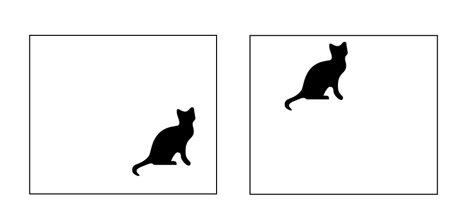
Translation symmetry: Same object in different locations.
For us, humans, it does not matter if a cat is in the right lower corner of it is somewhere in the top part of an image. In both cases we find a cat. So we can say that our human cat detector is translation invariant.
However, if we look at the architecture of a typical fully-connected network, we may realize that there is actually nothing that prevents this network to work correctly only on some part of an image. The question we ask: Is there a way to make a neural network translation invariant?
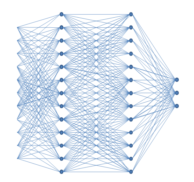
Fully-connected neural network with two hidden layers. Image credit: Wikimedia.
Let us take a closer look at the cat image. Soon we realize that pixels representing cat's head are more contextually related to each other than they are related to pixels representing cat's tail. Therefore, we also want to make our neural network sparse so that neurons in the next layer are connected only to the relevant neighboring pixels. This way, each neuron in the next layer would be responsible only for a small feature in the original image. The area that a neuron "sees" is called a receptive field.
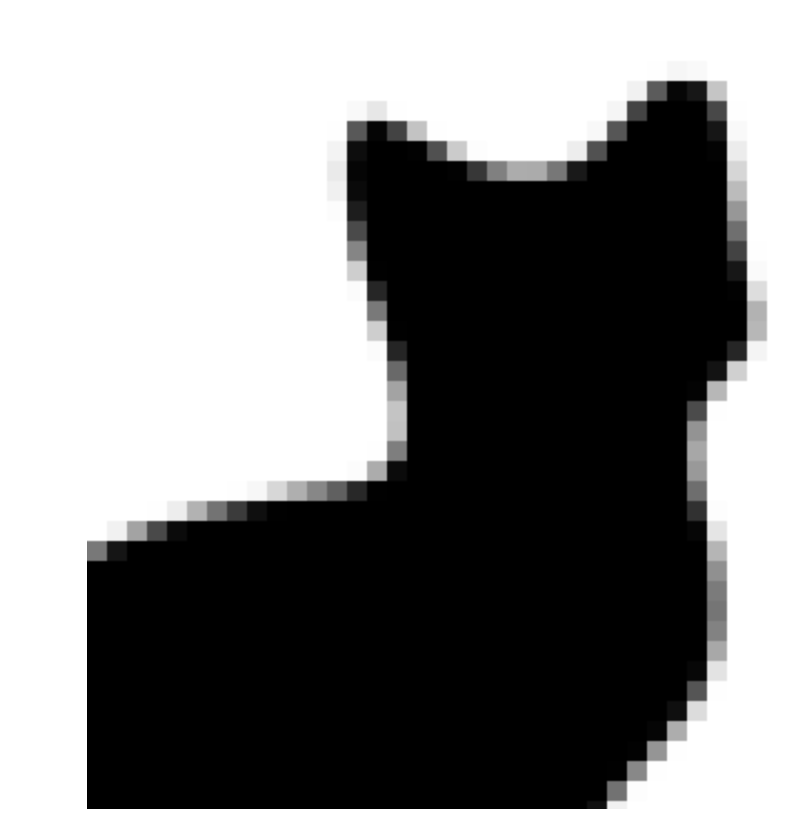
Neighboring pixels give more relevant information than distant ones. Zoom into the cats figure.
Convolutional neural networks (CNNs) or simply ConvNets were designed to address those two issues: translation symmetry and image locality. First, let us give an intuitive explanation of a convolution operator.
You may not be aware, but it is very likely you have already encountered convolution filters. Recall when you have first played with a (raster) graphics editor like GIMP or Photoshop. Probably you have been delighted obtaining effects such as sharpening, blur, or edge detection. If you haven't, then you probably should :). The secret of all those filters is the convolutional application of an image kernel. The image kernel is typically a 3×3 matrix such as below.
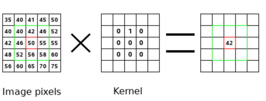
A single convolution step: Dot product between pixel values and a kernel. Image credit: GIMP.
Here is shown a single convolution step. This step is a dot product between the kernel and pixel values. Since all the kernel values except the second one in the first row are zeros, the result is equal to the second value in the first row of the green frame, i.e. 40⋅0+42⋅1+46⋅0+…+58⋅0=42. The convolution operator takes an image and acts within the green "sliding window"1 to perform dot product over every part of that image. The result is a new, filtered image. Mathematically, the (discrete) convolution operator (∗) between an image 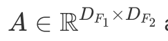 and a kernel
 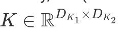 can be formalized as
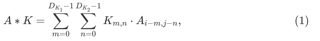
where 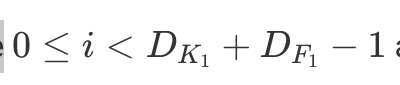 and
and  To better understand how convolution with a kernel changes the original image, you can play with different image kernels.
What is the motivation behind the sliding window/convolution operator approach? Actually, it has a biological background. In fact, human eye has a relatively narrow visual field. We perceive objects as a whole by constantly moving eyes around them. These rapid eye movements are called saccades. Therefore, convolution operator may be regarded as a simplified model of image scanning that occurs naturally. The important point is that convolutions achieve translation invariance thanks to the sliding window method. Moreover, since every dot product result is connected - through the kernel - only to a very limited number of pixels in the initial image, convolution connections are very sparse. Therefore, by using convolutions in neural networks we achieve both translation invariance and connection sparsity. Let us see how that works in practice.
Convolutional Neural Network Architecture
An interesting property of convolutional layers is that if the input image is shifted, the feature map output will be shifted by the same amount, but it will be left unchanged otherwise. This property is at the basis of the robustness of convolutional networks to shifts and distortions of the input.
Once a feature has been detected, its exact location becomes less important. Only its approximate position relative to other features is relevant.
Lecun et al. Gradient-based learning applied to document recognition (1998)
The prototype of what we call today convolutional neural networks has been first proposed back in late 1970s by Fukushima. There were proposed many unsupervised and supervised training methods, but today CNNs are trained almost exclusively with backpropagation. Let us take a look at one of the famous ConvNet architectures known as LeNet-5.
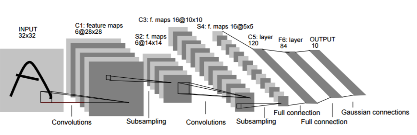
LeNet-5 architecture from Lecun et al. Gradient-based learning applied to document recognition.
The architecture is very close to modern CNNs. LeNet-5 was designed to perform handwritten digit recognition from 32×32 black and white images. The two main building blocks, as we call them now, are a feature extractor and a classifier.
With local receptive fields neurons can extract elementary visual features such as oriented edges, endpoints, corners...
Lecun et al. Gradient-based learning applied to document recognition (1998)
The feature extractor consists of two convolutional layers. The first convolutional layer has six convolutional filters with 5×5 kernels. Application of those filters with subsequent bias additions and hyperbolic tangent activations2 produces feature maps, essentially new, slightly smaller (28×28) images. By convention, we describe the result as a volume of 28×28×6. To reduce the spatial resolution, a subsampling is then performed3. That outputs 14×14×6 feature maps.
All the units in a feature map share the same set of 25 weights and the same bias, so they detect the same feature at all possible locations on the input.
Lecun et al. Gradient-based learning applied to document recognition (1998)
The next convolutions round results already in 10×10×16 feature maps. Note that unlike the first convolutional layer, we apply 5×5×6 kernels. That means that each of sixteen convolutions simultaneously processes all six feature maps obtained from the previous step. After subsampling we obtain a resulting volume of 5×5×16.
The classifier consists of three densely connected layers with 120, 84, and 10 neurons each. The last layer provides a one-hot-encoded4 answer. The slight difference from modern archictures is in the final layer, which consists of ten Euclidean radial basis function units, whereas today this would be a normal fully-connected layer followed by a softmax layer.
It is important to understand that a single convolution filter is able to detect only a single feature. For instance, it may be able to detect horizontal edges. Therefore, we use several more filters with different kernels to have get features such as vertical edges, simple textures, or corners. As you have seen, the number of filters is typically represented in ConvNet diagrams as volume. Interestingly, layers deeper in the network will combine the most basic features detected in the first layers into more abstract representations such as eyes, ears, or even complete figures. To better understand this mechanism let us inspect receptive fields visualization below.
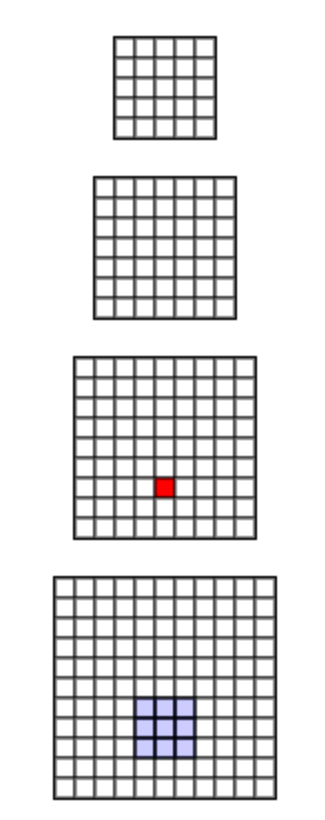
Receptive field visualization derived from Arun Mallya. Hover the mouse cursor over any neuron in top layers to see how extends its receptive field in previous (bottom) layers.
As we can see by checking neurons in last layers, even a small 3×3 receptive field grows as one moves towards first layers. Indeed, we may anticipate that "deeper" neurons will have better overall view on what happens in the image.
The beauty and the biggest achievement of deep learning is that filter kernels are self-learned by the network5, achieving even better accuracies compared to human-engineered features. A peculiarity of convolutional layers is that the result is obtained after repetitive application of a small number of weights as defined by a kernel. Thanks to this weight sharing, convolutional layers have drastically reduced number of trainable parameters6, compared to fully-connected layers.
Convolution Types
I decided to include this section for curious readers. If this is the first time you encounter CNNs, feel free to skip the section and revisit it later.
There is a lot of hype around convolutions nowadays. However, it is not made clear that low-level convolutions for computer vision are often different from those exploited by ConvNets. Yet, even in ConvNets there is a variety of convolutional layers inspired by Inception ConvNet architecture and shaped by Xception and Mobilenet works. I believe that you deserve to know that there exist multiple kinds of convolutions applied in different contexts and here I shall provide a general roadmap7.
Computer Vision-Style Convolution
 Low-level computer vision (CV), for instance graphics editors, typically operate one, three, or four channels images (e.g. red, green, blue, and transparency). An individual kernel is typically applied to each channel. In this case, usually there are as many resulting channels as there are channels in the input image. A special case of this style convolution is when the same convolution kernel is applied to each channel (e.g. blurring). Sometimes, resulting channels are summed producing a one-channel image (e.g. edge detection).
LeNet-like Convolution
A pure CV-style convolution is different from those in ConvNets due to two reasons: (1) in CV kernels are manually defined, whereas the power of neural networks comes from training, and (2) in neural networks we build a deep structure by stacking multiple convolutions on top of each other. Therefore, we need to recombine the information coming from previous layers. That allows us to train higher-level feature detections8. Finally, convolutions in neural networks may contain bias terms, i.e. constants added to results of each convolution.
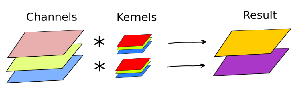
Recombination of features coming from earlier layers was previously illustrated in LeNet-5 example. As you remember, in the second convolutional layer we would apply 3D kernels of size 5×5×6 computing dot products simultaneously on all six feature maps from the first layer. There were sixteen different kernels thus producing sixteen new channels.
Each pixel in the feature map is obtained as a dot product between the RGB color channels and the sliding kernel. Image credit: Wikimedia. Convolution filter with three input channels. Each pixel in the feature map is obtained as a dot product between the RGB color channels and the sliding kernel. Image credit: Wikimedia.
To summarize, a single LeNet-like convolution operates simultaneously on all input channels and produces a single channel. By having an arbitrary number of kernels, any number of output channels is obtained. It is not uncommon to operate on volumes of 512 channels! The computation cost of such convolution is 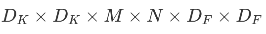 DK×DK×M×N×DF×DF where M is the number of input channels, N is the number of output channels,
  is the kernel size and
  is the feature map size9.
Depthwise Separable Convolution
LeNet-style convolution requires a large number of operations. But do we really need all of them? For instance, can spatial and cross-channel correlations be somehow decoupled? The Xception paper largely inspired by Inception architecture shows that indeed, one can build more efficient convolutions by assuming that spatial correlations and cross-channel correlations can be mapped independently. This principle was also applied in Mobilenet architectures.
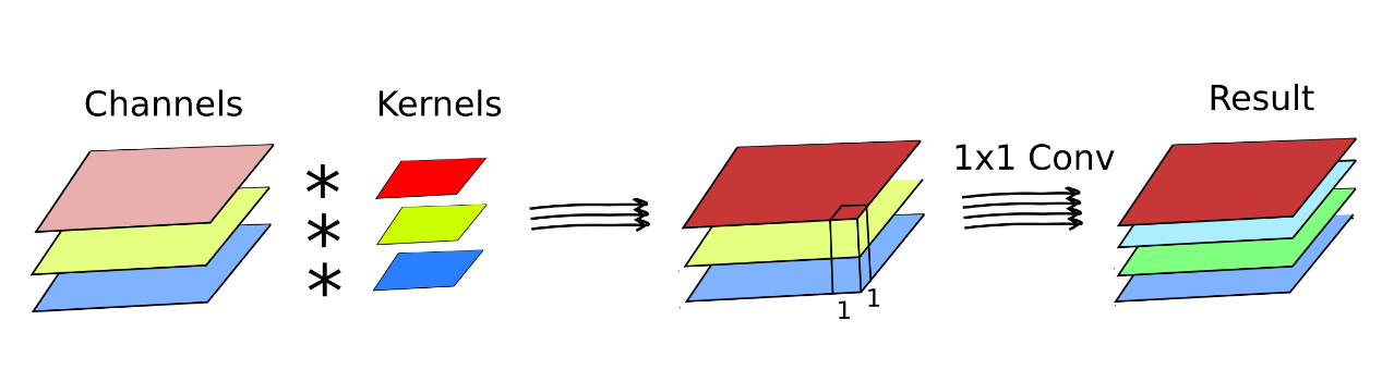
The depthwise separable convolution works the following way. First, like in low-level computer vision, individual kernels are applied to each individual channel. Then, after optional activation10, there is another convolution, but this time exclusively in-between channels. That is typically achieved by applying a 1×1 convolution kernel. Finally, there is a (ReLU) activation.
This way, depthwise separable convolution has two distinct steps: a space-only convolution and a channel recombination. This reduces the number of operations to 
To summarize, the main difference between low-level image processing (Photoshop) and neural networks is that image processing operates on lots of pixels, but the image depth remains unchanged (three-four channels). On the other hand, convolutional neural networks tend to operate on images of moderate width and height (e.g. 230×230 pixels), but can achieve depth of thousands of channels, while simultaneously decreasing the number of "pixels" in feature maps towards to the end of processing pipeline.
Implementing Convolutional Networks in Haskell
Today, we will implement and train a convolutional network inspired by LeNet-5. We will witness that indeed this ConvNet has about twice lower error on the MNIST handwritten digit recognition task, while being four times smaller compared to the previous model! The source code from this post is available on Github.
Convolutional Layer Gradients
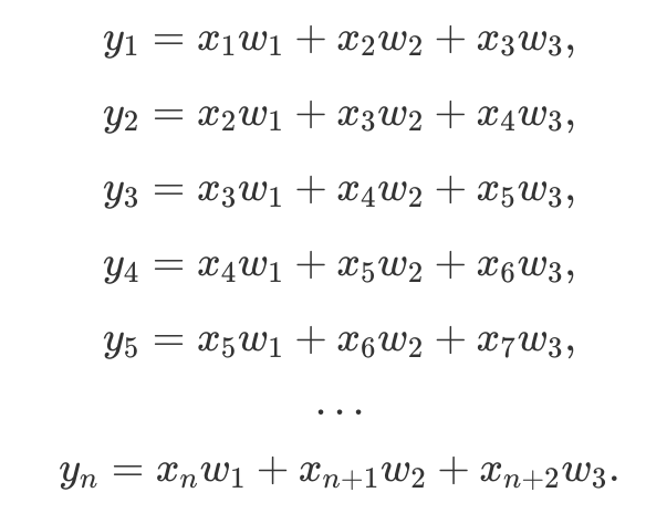
First of all, we need to know how to obtain convolutional layer gradients. Although convolution in neural networks is technically performed by the cross-correlation operator11, this does not matter since kernel parameters are learnable. To understand gradient derivation, let us take a look at the cross-correlation operation in single dimension:
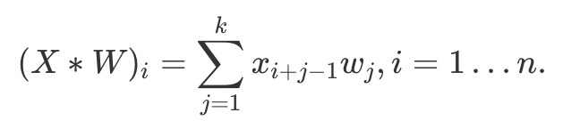
For instance, if we fix 1D kernel W size to be k=3, equation above would simply mean that vector 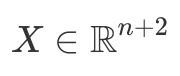 produces an output
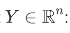
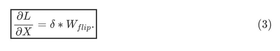
 Denoting error from the previous layer as δ, convolutional layer gradients w.r.t. input X are
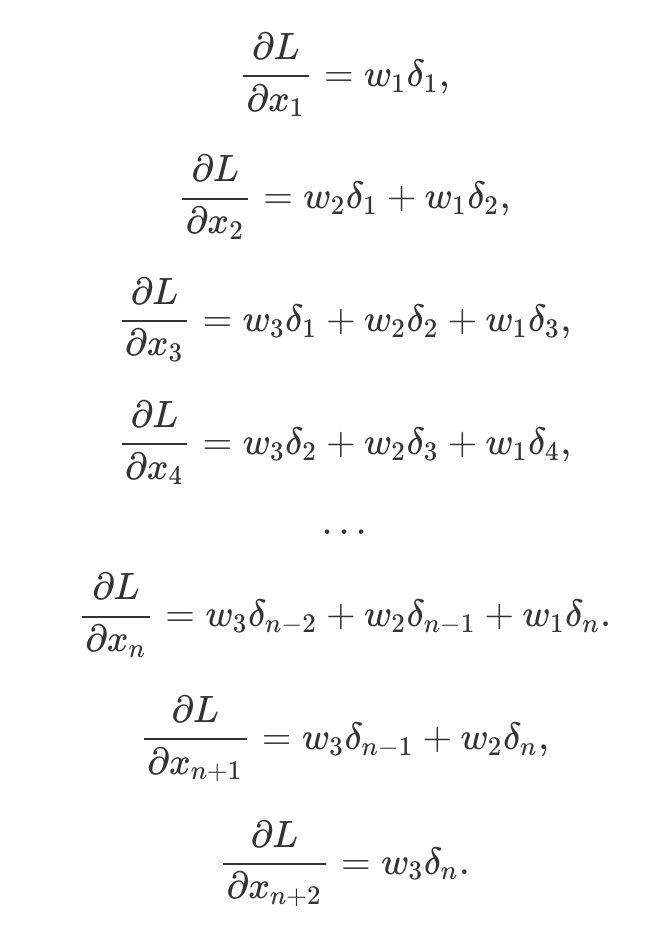
So it can be seen that it is a cross-correlation operation again, but with flipped kernel. Hence
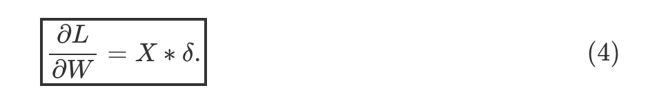
Similarly, gradients w.r.t. kernel W are computed as
 Thus we have yet another cross-correlation
These formulas will become handy when implementing the backward pass from convolutional layers.
Convolutions in Haskell
First, let us start with two most relevant imports: modules from array library massiv and automatic differentiation tools from backprop.
-- Multidimensional arrays to store learnable
-- parameters and represent image data
import           Data.Massiv.Array hiding ( map, zip, zipWith, flatten )
import qualified Data.Massiv.Array as A
-- Automatic heterogeneous back-propagation library
import           Numeric.Backprop
Let us brush up our data structures to match our convolutional needs. First, we need to represent a batch of images. We will use the following convention: batch size × channels × height × width. For instance, if we have a batch of 16 RGB images with dimensions 32 × 32 , then we get a volume of 16 × 3 × 32 × 32. Here we have a Volume4 type:
type Volume4 a = Array U Ix4 a
It is just an alias to a four-dimensional unboxed Array coming from the massiv package. In deep learning frameworks those n-dimensional arrays are conventionally called tensors. Note that during transformation in a neural network, the shape of data will change, except the batch dimension that will always remain the same. Similarly, we need a way to represent our convolutional filters. In LeNet, for instance, we can represent the first convolutional layer as a volume of 6×1×5×5. In order to be able to distinguish between parameter and data volumes, we will introduce Conv2d data structure:
data Conv2d a = Conv2d { _kernels :: !(Volume4 a) }
Note that for the sake of simplicity we decided not to implement biases. As previously, Linear will represent fully-connected layer parameters:
data Linear a = Linear { _weights :: !(Matrix a)
                       , _biases :: !(Vector a)
                       }
As usual, type parameter a means that we may later decide whether we need a Float, a Double or some other weights encoding. Now, we have everything to describe learnable parameters (weights) in LeNet:
data LeNet a =
    LeNet { _conv1 :: !(Conv2d a)
          , _conv2 :: !(Conv2d a)
          , _fc1 :: !(Linear a)
          , _fc2 :: !(Linear a)
          , _fc3 :: !(Linear a)
          }
Now, it becomes obvious that with every new layer type managing backpropagation data structures as we did on Days 2 and 4 quickly becomes tedious. Moreover, last time when we introduced a Batchnorm1d layer, our forward-backward pass function already oversized 100 lines of code. Today, we will make use of the backprop library introduced on Day 3 to better structure our project. Thus, LeNet can be represented as a differentiable function lenet, which is nothing more than a composition of other functions aka neural network layers:
lenet :: (Reifies s W)
      => BVar s (LeNet Float)
      -> Volume4 Float  -- ^ Batch of images
      -> BVar s (Matrix Float)
lenet l = constVar

          -- Feature extractor
          -- Layer (layer group) #1
          ~> sameConv2d (l ^^. conv1)
          ~> relu
          ~> maxpool
          -- Layer #2
          ~> validConv2d (l ^^. conv2)
          ~> relu
          ~> maxpool

          ~> flatten

          -- Classifier
          -- Layer #3
          ~> linear (l ^^. fc1)
          ~> relu
          -- Layer #4
          ~> linear (l ^^. fc2)
          ~> relu
          -- Layer #5
          ~> linear (l ^^. fc3)
This description pretty much talks for itself. The (~>) operator is a function composition, i.e. f ~> g = \x -> g(f(x)). This could be written in other forms, though. We prefer the so-called pointfree notation:
(~>) :: (a -> b) -> (b -> c) -> a -> c
f ~> g = g. f
That simply reverses the order of composition, i.e. first is applied f, and only then g12. I find this "backward composition" notation consistent with major neural network frameworks. Compare how an equivalent network can be represented in PyTorch:
import torch.nn as nn

class LeNet(nn.Module):
    def __init__(self, num_classes=10):
        super(LeNet, self).__init__()
        # Feature extractor: a (sequential) composition of convolutional,
        # activation, and pooling layers
        self.features = nn.Sequential(
            nn.Conv2d(1, 6, kernel_size=5, stride=1, padding=2, bias=False),
            nn.ReLU(),
            nn.MaxPool2d(kernel_size=2, stride=2),
            nn.Conv2d(6, 16, kernel_size=5, stride=1, padding=0, bias=False),
            nn.ReLU(),
            nn.MaxPool2d(kernel_size=2, stride=2)
        )

        # Classifier: a composition of linear and activation layers
        self.classifier = nn.Sequential(
            nn.Linear(16 * 5 * 5, 120, bias=True),
            nn.ReLU(),
            nn.Linear(120, 84, bias=True),
            nn.ReLU(),
            nn.Linear(84, num_classes, bias=True)
        )

    # Composition of feature extractor and classifier
    def forward(self, x):
        x = self.features(x)
        # Flatten
        x = x.view(x.size(0), -1)
        x = self.classifier(x)
        return x
Despite some noise in the Python code above13, we see that nn.Sequential object acts simply as a function composition with (~>) combinators. Now, let us return back to lenet signature:
lenet :: (Reifies s W)
      => BVar s (LeNet Float)
      -> Volume4 Float  -- ^ Batch of images
      -> BVar s (Matrix Float)
We have already seen the BVar s ("backprop variable") type meaning that we deal with a differentiable structure. The first argument has type BVar s (LeNet Float). That conventionally means that LeNet is the model optimized by backpropagation and shortly we will show how to achieve that. The second function argument is a batch of images (Volume4), and finally the result is a bunch of vectors (Matrix) containing classification results performed by our model.
Functions constVar and (^^.) are special ones. Both are coming from the Numeric.Backprop import. The first function "lifts" a batch to be consumed by the sequence of differentiable functions. The second one (^^.) allows us to conveniently access records from our LeNet data type. For instance, sameConv2d (l ^^. conv1) means that sameConv2d has access to the _conv1 field.
Layers known from the previous days (linear, ReLU) will be reused in accordance to backprop conventions. What is left to implement are sameConv2d, validConv2d, and maxpool layers. To be able to do that simply and efficiently we will learn a neat tool called stencils.
Fun With Stencils
Let us come back to 1D convolution from Equation (2). If we look closer, we notice a pattern in convolution/cross-correlation, i.e. 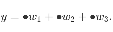 Indeed, every time we multiply the same set of weights and the only thing that changes is source data (masked with bullets above). Therefore, to implement convolutions we only need to define some sort of pattern that processes given points. This fixed pattern applied to array elements is called a stencil. The stencil convolution approach can be also used to perform subsampling operations, e.g. max pooling. Moreover, the method allows for efficient data parallelism.
Previously, we have introduced Massiv library featuring parallel arrays computation. This library was preferable to hmatrix due to two reasons: multidimensional arrays and parallel computation. Today, we have yet one more reason: stencils. Good news: massiv already implements them for us! Those are based on this work.
First, we warm up with a 1D cross-correlation from Equation (2). Suppose, we have a "delay" kernel [1,0,0]. Here is how this can be applied in an interactive shell (aka REPL):
> import Data.Massiv.Array
> type Vector a = Array U Ix1 a  -- Convenience alias
> k = fromList Par [1, 0, 0] :: Vector Int
> sten = makeCorrelationStencilFromKernel k
> dta = fromList Par [1, 2, 5, 6, 2, -1, 3, -2] :: Vector Int
> mapStencil (Fill 0) sten dta
Array DW Par (Sz1 8)
  [ 0, 1, 2, 5, 6, 2, -1, 3 ]
Note that the first value was replaced with zero since we have applied mapStencil (Fill 0) that uses zero-filling padding strategy to preserve the size of the array. Our array was processed to look internally like this: [0,1,2,5,6,2,−1,3,−2,0], with fake zeros inserted. Alternatively, we could use applyStencil noPadding as below:
> applyStencil noPadding sten dta
Array DW Par (Sz1 6)
  [ 1, 2, 5, 6, 2, -1 ]

> dta' = fromList Par [0, 1, 2, 5, 6, 2, -1, 3, -2, 0] :: Vector Int
> applyStencil noPadding sten dta'
Array DW Par (Sz1 8)
  [ 0, 1, 2, 5, 6, 2, -1, 3 ]
Here is a more interesting computer vision example. For comparison, we define an identity (no transformation) stencil and a box stencil (blurring effect). The identity kernel has one in its center (coordinate 0 :. 0) and zeroes everywhere else. The box transformation computes averaged value over nine neighboring pixels including the center pixel itself (see also this for more information), therefore the kernel has weights 1/9 everywhere.
import Data.Massiv.Array
import Data.Massiv.Array.IO
import Graphics.ColorSpace

identity :: Elevator a => Stencil Ix2 (Pixel RGB a) (Pixel RGB a)
identity =
  makeStencil sz c $ \get -> get (0 :. 0)
  -- `get` is a function that receives a coordinate relative to the
  -- stencil's center, i.e. (0 :. 0) is the center itself.
  where
    sz = Sz (3 :. 3)  -- Kernel size: 3 x 3
    c = 1 :. 1  -- Center coordinate
{-# INLINE identity #-}

box :: (Elevator a, Fractional a) => Stencil Ix2 (Pixel RGB a) (Pixel RGB a)
box =
  makeStencil sz c $ \get ->
    ( get  (-1 :. -1) + get  (-1 :. 0) + get (-1 :. 1)
    + get  (0 :. -1) + get  (0 :. 0) + get (0 :. 1)
    + get  (1 :. -1) + get  (1 :. 0) + get (1 :. 1)) / 9
  where
    sz = Sz (3 :. 3)
    c = 1 :. 1
{-# INLINE box #-}

main :: IO ()
main = do
  frog <- readImageAuto "files/frog.jpg" :: IO (Image S RGB Double)

  -- Identity transformation
  writeImageAuto "files/frog_clone.png" $ computeAs S (mapStencil Edge identity frog)
  -- Box filtering (blur)
  writeImageAuto "files/frog_blurred.png" $ computeAs S (mapStencil Edge box frog)
In main function, we load an image and apply those two stencils. All we need to do is to specify the stencil pattern, i.e. convolution kernel, and massiv takes care to apply it. This is what we get:
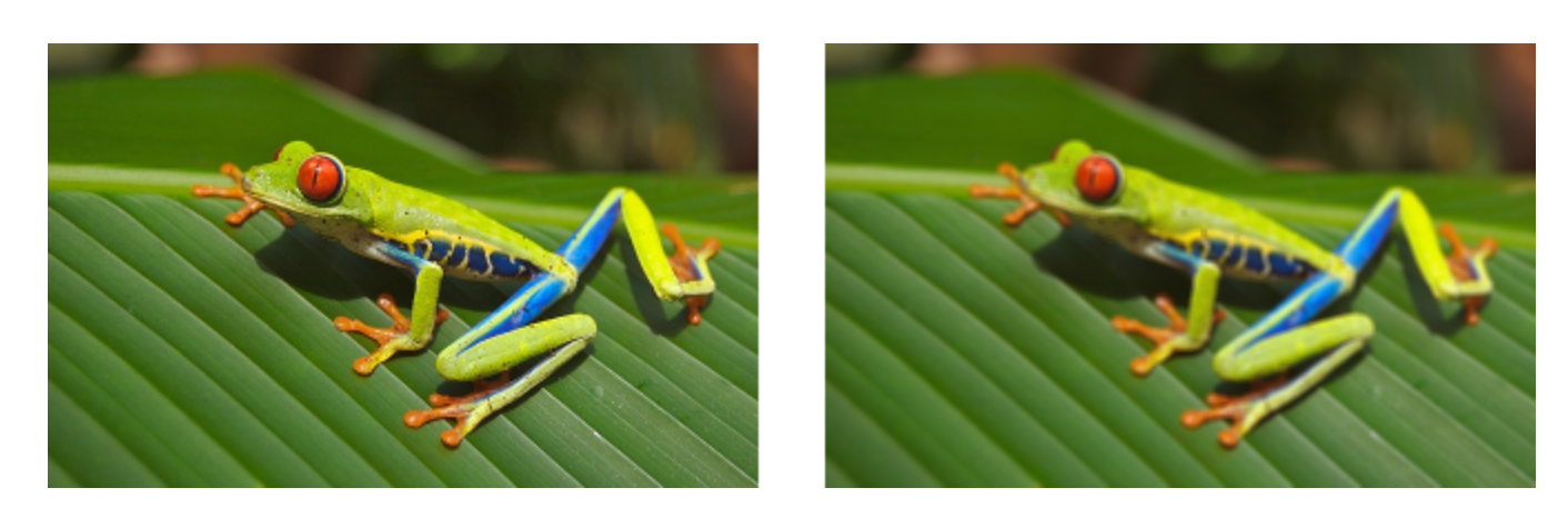
Original frog (left) and blurred (right). Image credit. While in the last example above we have defined stencils manually with makeStencil, in practice we may prefer to use
makeCorrelationStencilFromKernel
  :: (Manifest r ix e, Num e) => Array r ix e -> Stencil ix e e
The function has a single argument, stencil's kernel.
Convolutional Layers With Stencils
Before actually diving into implementation, we have to understand that convolution decreases the number of "pixels" in the image, similar to the "delayed" 1D kernel above. Moreover, some information next to the image border is lost due to the fact that the sliding window "visits" bordering pixels less than those closer to the center. To avoid the information loss, often the area around the image is "padded" (filled) with zeros. Thus we can perform a "same" convolution, i.e. one that does not change the convolved dimensions. As of version 0.4.3, Massiv stencils already support different padding modes. In case of LeNet 5×5 kernels, we define padding of 2 pixels on every side (top, right, bottom, and left) using top left and bottom right corners:
sameConv2d = conv2d (Padding (Sz2 2 2) (Sz2 2 2) (Fill 0.0))
"Valid" convolution is a convolution with no padding:
validConv2d = conv2d (Padding (Sz2 0 0) (Sz2 0 0) (Fill 0.0))
In both cases, we will use generic conv2d function with a padding argument. Supporting automatic differentiation, our conv2d combines both forward and backward passes:
conv2d :: Reifies s W
       => Padding Ix2 Float
       -> BVar s (Conv2d Float)
       -> BVar s (Volume4 Float)
       -> BVar s (Volume4 Float)
The signature tells us that it is a differential function that takes a padding, Conv2d parameters, and a batch of images Volume4 and produces another batch of images. The most efficient way to define the function is to manually specify both forward and backward passes; although it is also possible to specify only the forward pass composing smaller functions operating on BVars and letting backprop to figure out their gradients. The general pattern in backprop is to provide the forward pass (Conv2d w) x -> ... and the backward pass using a lambda expression containing previously computed gradients dz as an argument. Those forward and backward passes are glued together with liftOp2. op2 (or liftOp1. op1 for layers with no learnable parameters) as below:
conv2d p = liftOp2. op2 $ \(Conv2d w) x ->
  (conv2d_ p w x, \dz -> let dw = conv2d'' p x dz
                             -- ... Compute padding p1
                             dx = conv2d' p1 w dz
                         in (Conv2d dw, dx) )
Now, forward pass is a cross-correlation between the input channels and a kernel set from the filter bank. Recall that the number of kernel sets defines the number of output channels. We simultaneously perform cross-correlation operations on all images in the batch, therefore we concatenate the results over the channel dimension 3.
conv2d_ pad w x = res
  where
    -- Some code omitted for simplicity

    -- Create a stencil ("sliding window") from the given set
    -- in the filter bank
    sten = makeCorrelationStencilFromKernel. resize' (Sz4 1 cin w1 w2). (w !>)

    -- For each kernel set, create and run stencils on all images in the batch.
    -- Finally, concatenate (append) the results over the channel dimension
    res = foldl' (\prev ch -> let conv = computeAs U $ applyStencil pad4 (sten ch) x
                              in computeAs U $ append' 3 prev conv) empty [0..cout - 1]
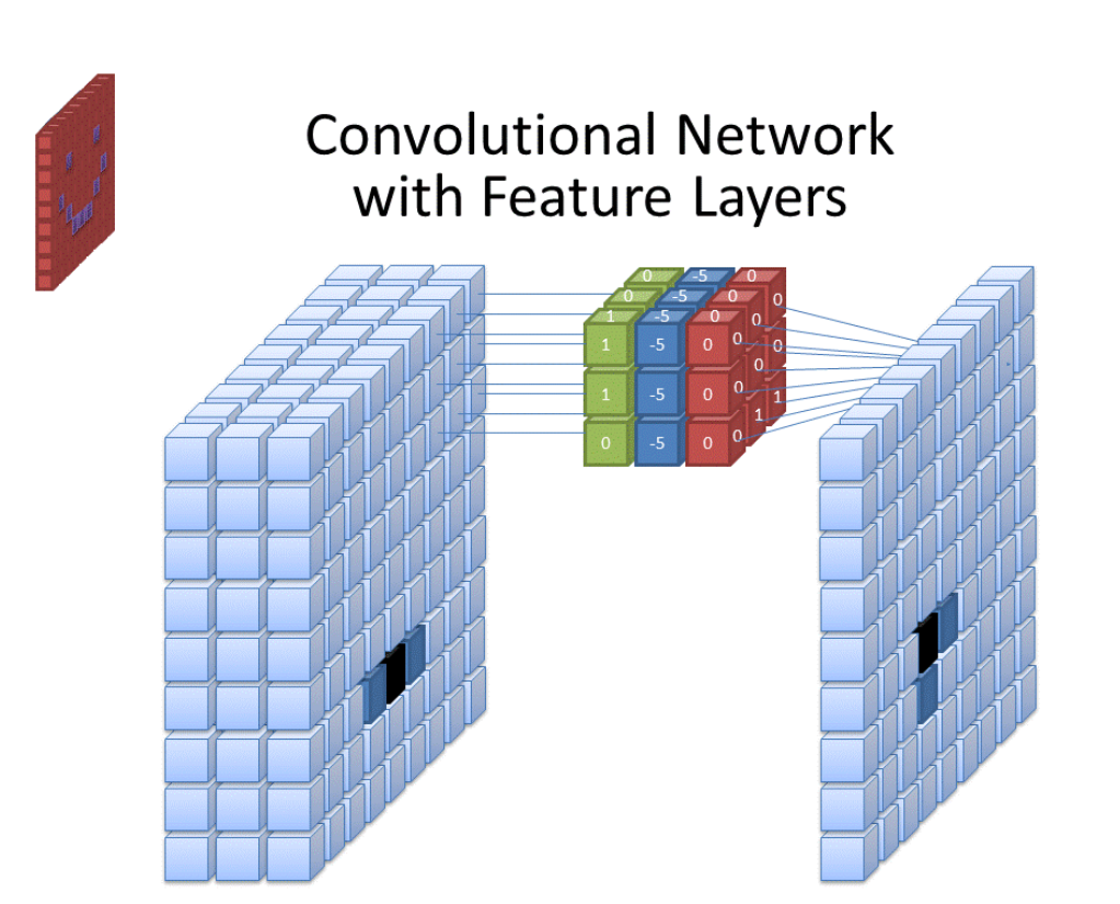
To better illustrate how this works on a batch of images, here is a visualization what is going on in the first convolutional layer.
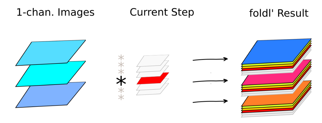
Folding over six filter sets in the first convolutional layer. Currently active convolutional filter set (highlighted in red) contributes to so far processed results (in color) on the right. Folding over six filter sets in the first convolutional layer. Currently active convolutional filter set (highlighted in red) contributes to so far processed results (in color) on the right.
In MNIST we have black and white images, thus a single-channel input. During each step in foldl', a single filter is applied to all images. There are six filters hence resulting in six new channels in each convolved image on the right. A similar operation is performed in the second convolutional layer, this time resulting in 16-channel images (see also Convolution Types. LeNet-like Convolution above for the illustration on a single image). Below is a Python/NumPy equivalent of foldl'/applyStencil combo from above.
import numpy as np

# ... Get current batch, stride, and padding parameters
# ... Using those parameters, determine
# output image width, height, and number of channels

# Initialize resulting array
res = np.zeros([len(batch), out_channels, out_im_height, out_im_width])

# Iterate over all four dimensions
for i in range(len(batch)):
    for j in range(out_im_height):
        for k in range(out_im_width):
            for c in range(out_channels):
                # Define the sliding window position
                y1 = j * stride
                y2 = y1 + kernel_height
                x1 = k * stride
                x2 = x1 + kernel_width
                im_slice = batch[i, :, y1:y2, x1:x2]

                # Get current channel weights
                Wcur = W[:,c,:,:]

                # Out pixel = dot product
                res[i, c, j, k] = np.sum(im_slice * Wcur)

return res
Now that we have accomplished convolution in the forward direction, we need to compute gradients for the backward pass.
Gradients Are Also Convolutions
The image plane gradients are obtained by formulas (3) and (4). However, in practice we also have to take into account that we deal with multiple images that have multiple channels. In fact, I leave it to you to figure out exact formulas. Those can be inferred from Haskell equations below. Yes, any Haskell line is already written in a mathematical notation. That is essentially what Haskell "purity" is about. You might have realized by now that programming in Haskell is all about finding your own patterns. Now, let us compute gradients w.r.t. input 
conv2d' p w dz = conv2d_ p w' dz
  where
    w' = (compute. rot180. transposeInner) w

    -- Rotate kernels by 180 degrees. This is expressed in terms
    -- of tensor reversal along width and height dimensions.
    rot180 = reverse' 1. reverse' 2
Let us remind that these compute functions evaluate delayed arrays into actual representation in memory. Please do not hesitate to find reverse and transposeInner in massiv documentation. Finally, here we have gradients w.r.t. convolution kernel weights 
conv2d''
  :: Padding Ix2 Float -> Volume4 Float -> Volume4 Float -> Volume4 Float
-- Iterate over images in a batch
conv2d'' p x dz = res  -- computeMap (/fromIntegral bs) res
  where
    -- Batch size
    Sz (bs :> _) = size x

    -- Code omitted

    res = foldl' (\acc im ->
      let cur = _conv2d'' p (compute $ dzd !> im) (compute $ xd !> im)
       in acc + cur) base [1..bs-1]
We simply accumulate gradients from individual images in the batch using left strict fold. Finally, we generalize Equation (4) to get those transformations:

_conv2d'' :: Padding Ix2 Float
          -> Volume Float  -- ^ Gradients \delta (dz)
          -> Volume Float  -- ^ X
          -> Volume4 Float  -- ^ dL/dW
_conv2d'' (Padding (Sz szp1) (Sz szp2) pb) dz x = ...
More Stencils: Max Pooling Layers
Stencils are handy not only for convolutional layers. Another use case are pooling (subsampling) layers. To be able to perform max pooling, first we have to define the corresponding stencil pattern (or just use maxStencil from the library instead).

maxpoolStencil2x2 :: Stencil Ix4 Float Float
maxpoolStencil2x2 = makeStencil (Sz4 1 1 2 2) 0 $ \ get ->
  let max4 x1 x2 x3 x4 = max (max (max x1 x2) x3) x4
   in max4 <$> get (0 :> 0 :> 0 :. 0)
           <*> get (0 :> 0 :> 1 :. 1)
           <*> get (0 :> 0 :> 0 :. 1)
           <*> get (0 :> 0 :> 1 :. 0)
Here max4 is a function that receives four values and computes the maximal one. This function is applied to a patch of four neighboring pixels. Do not forget that we operate in a 4D space, therefore each point in the given patch has four coordinates. Here is how we interpret a coordinate:

 (0 :> 0 :> 0 :. 0)
  ^    ^    ^    ^
  4    |    |    1
       3    2
1 and 2 are coordinates in the image plane,
3 is the channel dimension, and
4 is the batch dimension.
Note the :. and :> operators. The first one :. constructs a coordinates (index) "list" with two elements and :> just adds more coordinates for higher dimensions. To learn more about <$> and <*> functions, see Applicative Functors.

We would like to have non-overlapping sliding windows in max pooling, therefore, we want to use
2
×
2
 stride in the image plane. However, we would like to perform the same operation over every channel in every image. Therefore, we use computeWithStride and the stride is 1 :> 1 :> 2 :. 2 (
batch dim
×
channel dim
×
height
×
width
). Note that we do not want any padding since the goal of pooling is actually to reduce the number of pixels: four times in this case.

maxpool_ :: Volume4 Float -> Volume4 Float
maxpool_ = computeWithStride (Stride (1 :> 1 :> 2 :. 2)).
             applyStencil noPadding maxpoolStencil2x2
Finally, we compute gradients using pixels that had maximal values in the forward pass. And we obtain a differentiable maxpool function lifting forward-backward passes with liftOp1. op1:

maxpool :: Reifies s W
        => BVar s (Volume4 Float)
        -> BVar s (Volume4 Float)
maxpool = liftOp1. op1 $ \x ->
  let out = maxpool_ x
      s = Stride (1 :> 1 :> 2 :. 2)
      outUp = computeAs U $ zoom s out
      maxima = A.zipWith (\a b -> if a == b then 1 else 0) outUp x
  in (out, \dz -> let dzUp = computeAs U $ zoom s dz
                  -- Elementwise product
                  in maybe (error $ "Dimensions problem") compute (maxima .*. delay dzUp))
Putting It All Together
First, we fetch the MNIST data and randomly generate the initial model:

main :: IO ()
main = do
  trainS <- mnistStream 64 "data/train-images-idx3-ubyte" "data/train-labels-idx1-ubyte"
  testS <- mnistStream 1000 "data/t10k-images-idx3-ubyte" "data/t10k-labels-idx1-ubyte"

  net <- randNetwork
As previously, data streams are loaded from binary MNIST files; however, the initial model generation has to take into account the new structure, LeNet.

randNetwork :: IO (LeNet Float)
randNetwork = do
  -- Generate a new conv layer weights:
  -- 6 out channels, 1 input channel, kernel size: 5 x 5
  _conv1 <- randConv2d (Sz4 6 1 5 5)
  -- 16 out channels, 6 input channels, kernel size: 5 x 5
  _conv2 <- randConv2d (Sz4 16 6 5 5)
  let [i, h1, h2, o] = [16 * 5 * 5, 120, 84, 10]
  _fc1 <- randLinear (Sz2 i h1)
  _fc2 <- randLinear (Sz2 h1 h2)
  _fc3 <- randLinear (Sz2 h2 o)
  return $
    LeNet { _conv1 = _conv1
          , _conv2 = _conv2
          , _fc1 = _fc1
          , _fc2 = _fc2
          , _fc3 = _fc3
          }
Finally, we train our model

  -- ... `main` function
  net' <- train TrainSettings { _printEpochs = 1
                              , _lr = 0.01
                              , _totalEpochs = 30
                              } net (trainS, testS)
The train function is essentially a wraper around the sgd stochastic gradient descent function.

train TrainSettings { _printEpochs = printEpochs
                    , _lr = lr
                    , _totalEpochs = totalEpochs
                    } net (trainS, testS) = do
  (net', _) <- iterN (totalEpochs `div` printEpochs) (\(net0, j) -> do
    net1 <- sgd lr printEpochs net0 trainS

    -- ... Compute and print accuracies

    ) (net, 1)
  return net'
In sgd we compute gradients over a mini-batch and subtract them to optimize the model parameters.

sgd lr n net0 dataStream = iterN n epochStep net0
  where
    -- Fold over the stream of all batches
    epochStep net = S.foldl' _trainStep net dataStream
    -- Update gradients based on a single batch
    _trainStep net (x, targ) = trainStep lr x targ net
Now, the training step is a few lines of code thanks to Numeric.Backprop.gradBP function that applies the chain rule, thus replacing the entire pass function we had before.

trainStep
  :: Float  -- ^ Learning rate
  -> Volume4 Float  -- ^ Images batch
  -> Matrix Float  -- ^ Targets
  -> LeNet Float  -- ^ Initial network
  -> LeNet Float
trainStep lr !x !targ !n = n - lr * (gradBP (crossEntropyLoss x targ) n)
If we ever want to actually use our model to identify a handwritten digit, we call evalBP:

forward :: LeNet Float -> Volume4 Float -> Matrix Float
forward net dta = evalBP (`lenet` dta) net
Now, we compile and run our program:

$ ./run.sh
1 Training accuracy 10.4  Validation accuracy 10.3
2 Training accuracy 85.7  Validation accuracy 86.3
3 Training accuracy 95.9  Validation accuracy 96.2
4 Training accuracy 97.6  Validation accuracy 97.4
5 Training accuracy 98.4  Validation accuracy 98.1
6 Training accuracy 98.3  Validation accuracy 98.0
7 Training accuracy 99.0  Validation accuracy 98.8
8 Training accuracy 99.0  Validation accuracy 98.7
9 Training accuracy 99.1  Validation accuracy 98.7
...
26 Training accuracy 99.8  Validation accuracy 99.0
27 Training accuracy 99.8  Validation accuracy 98.7
28 Training accuracy 99.9  Validation accuracy 98.9
29 Training accuracy 99.7  Validation accuracy 98.6
30 Training accuracy 99.9  Validation accuracy 98.9
Thus, after 30 training epochs, we have obtained a
∼
1
%
 validation error, which is about twice as low compared to the simple fully-connected architecture. See the complete project on Github.

Model Parameters Comparison
Our three-layer model from Day 4 consumed

(
784
+
1
)
⋅
300
+
(
300
+
1
)
⋅
50
+
(
50
+
1
)
⋅
10
=
251
,
060
learnable parameters (not counting batchnorm parameters). In contrast, the convolutional neural network model that we have implemented today requires only

1

⋅
5
⋅
5
⋅
6
+
16
⋅
6
⋅
5
⋅
5
+
(
400
+
1
)
⋅
120
+
(
120
+
1
)
⋅
84
+
+
(
84
+
1
)
⋅
10
=
61
,
684

parameters.
Note also that
1

⋅
5
⋅
5
⋅
6
+
16
⋅
6
⋅
5
⋅
5
=
2
,
550
 are convolutional layers parameters, whereas the majority (
59
,
134
) reside in classifier's fully-connected layers.

Although, we did not apply batch normalization today, like was in the original LeNet, feel free to experiment with adding batchnorm layers. Please also note that there is a difference between batch normalization after convolution and after fully-connected layers (see the batchnorm article).

Citation
@article{penkovsky2019CNN,
 title   = "Convolutional Neural Networks Tutorial",
 author  = "Penkovsky, Bogdan",
 journal = "penkovsky.com",
 year    = "2019",
 month   = "November",
 url     = "https://penkovsky.com/neural-networks/day5/"
}
Summary
Convolutional neural networks aka ConvNets achieve translation invariance and connection sparsity. Thanks to weight sharing, ConvNets dramatically reduce the number of trained parameters. The power of ConvNet comes from training convolution filters, in contrast to manual feature engineering. In future posts, we will gain the power of GPU to face bigger challenges. We will save the planet. And we might even try to read someone's mind with convolutional networks. Stay tuned!

Acknowledgment
I would like to acknowledge Alexey Kuleshevich for his help with massiv array library, upon which this convolutional neural network was built.

Further reading
Learned today:

Interactive Image Kernels
Excellent tutorial on ConvNets
The Ancient Secrets of Computer Vision (online course)
Why I prefer functional programming
Efficient Parallel Stencil Convolution in Haskell
Deeper into neural networks:

LeNet-5 paper
Inception paper
Xception paper
Mobilenet paper