Day 3: Haskell Guide To Neural Networks

Now that we have seen how neural networks work, we realize that understanding of the gradients flow is essential for survival. Therefore, we will revise our strategy on the lowest level. However, as neural networks become more complicated, calculation of gradients by hand becomes a murky business. Yet, fear not young padawan, there is a way out! I am very excited that today we will finally get acquainted with automatic differentiation, an essential tool in your deep learning arsenal. This post was largely inspired by Hacker's guide to Neural Networks. For comparison, see also Python version.

Before jumping ahead, you may also want to check the previous posts:

Day 1: Learning Neural Networks The Hard Way

Day 2: What Do Hidden Layers Do? The source code from this guide is available on Github. The guide is written in literate Haskell, so it can be safely compiled.

Why Random Local Search Fails

Following Karpathy's guide, we first consider a simple multiplication circuit. Well, Haskell is not JavaScript, so the definition is pretty straightforward:

forwardMultiplyGate = (*)

Or we could have written

forwardMultiplyGate x y = x * y

to make the function look more intuitively f(x,y)=x⋅y. Anyway,

forwardMultiplyGate (-2) 3

returns -6. Exciting.

Now, the question: is it possible to change the input (x,y) slightly in order to increase the output? One way would be to perform local random search.

_search tweakAmount (x, y, bestOut) = do
  x_try <- (x + ). (tweakAmount *) <$> randomDouble
  y_try <- (y + ). (tweakAmount *) <$> randomDouble
  let out = forwardMultiplyGate x_try y_try
  return $ if out > bestOut
               then (x_try, y_try, out)
               else (x, y, bestOut)

Not surprisingly, the function above represents a single iteration of a "for"-loop. What it does, it randomly selects points around initial (x,y) and checks if the output has increased. If yes, then it updates the best known inputs and the maximal output. To iterate, we can use foldM :: (b -> a -> IO b) -> b -> [a] -> IO b. This function is convenient since we anticipate some interaction with the "external world" in the form of random numbers generation:

localSearch tweakAmount (x0, y0, out0) =
 foldM (searchStep tweakAmount) (x0, y0, out0) [1..100]

What the code essentially tells us is that we seed the algorithm with some initial values of x0, y0, and out0 and iterate from 1 till 100. The core of the algorithm is searchStep:

searchStep ta xyz _ = _search ta xyz

which is a convenience function that glues those two pieces together. It simply ignores the iteration number and calls _search. Now, we would like to have a random number generator within the range of [-1; 1). From the documentation, we know that randomIO produces a number between 0 and 1. Therefore, we scale the value by multiplying by 2 and subtracting 1:

randomDouble :: IO Double
randomDouble = subtract 1. (*2) <$> randomIO

The <$> function is a synonym to fmap. What it essentially does is attaching the pure function subtract 1. (*2) which has type Double -> Double, to the "external world" action randomIO, which has type IO Double (yes, IO = input/output)1.

A hack for a numerical minus infinity:

inf_ = -1.0 / 0

Now, we run localSearch 0.01 (-2, 3, inf_) several times:

(-1.7887454910045664,2.910160042416705,-5.205535653974539)
(-1.7912166830200635,2.89808308735154,-5.19109477484237)
(-1.8216809458018006,2.8372869694452523,-5.168631610010152)

In fact, we see that the outputs have increased from -6 to about -5.2. But the improvement is only about 0.8/100 = 0.008 units per iteration. That is an extremely inefficient method. The problem with random search is that each time it attempts to change the inputs in random directions. If the algorithm makes a mistake, it has to discard the result and start again from the previously known best position. Wouldn't it be nice if instead each iteration would improve the result at least by a little bit?

Automatic Differentiation

Instead of random search in random direction, we can make use of the precise direction and amount to change the input so that the output would improve. And that is exactly what the gradient tells us. Instead of manually computing the gradient every time, we can employ some clever algorithm. There exist multiple approaches: numerical, symbolic, and automatic differentiation. In his article, Dominic Steinitz explains the differences between them. The last approach, automatic differentiation is exactly what we need: accurate gradients with minimal overhead. Here, we will briefly explain the concept.

The idea behind automatic differentiation is that we explicitly define gradients only for elementary, basic operators. Then, we exploit the chain rule combining those operators into neural networks or whatever we like. That strategy will infer the necessary gradients by itself. Let us illustrate the method with an example.

Below we define both multiplication operator and its gradient using the chain rule, i.e.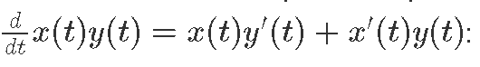

(x, x') *. (y, y') = (x * y, x * y' + x' * y)

The same can be done with addition, subtraction, division, and exponent:

(x, x') +. (y, y') = (x + y, x' + y')

x -. y = x +. (negate1 y)

negate1 (x, x') = (negate x, negate x')

(x, x') /. (y, y') = (x / y, (y * x' - x * y') / y^2)

exp1 (x, x') = (exp x, x' * exp x)

We also have constOp for constants:

constOp :: Double -> (Double,Double)
constOp x = (x, 0.0)

Finally, we can define our favourite sigmoid σ(x) combining the operators above:

sigmoid1 x = constOp 1 /. (constOp 1 +. exp1 (negate1 x))

Now, let us compute a neuron f(x,y)=σ(ax+by+c), where x and y are inputs and a, b, and c are parameters

neuron1 [a, b, c, x, y] = sigmoid1 ((a *. x) +. (b *. y) +. c)

Now, we can obtain the gradient of a in the point where a=1, b=2, c=−3, x=−1, and y=3:

abcxy1 :: [(Double, Double)]
abcxy1 = [(1, 1), (2, 0), (-3, 0), (-1, 0), (3, 0)]

neuron1 abcxy1
(0.8807970779778823,-0.1049935854035065)

Here, the first number is the result of the neuron's output and the second one is the gradient with respect to a Let us verify the math behind the result: 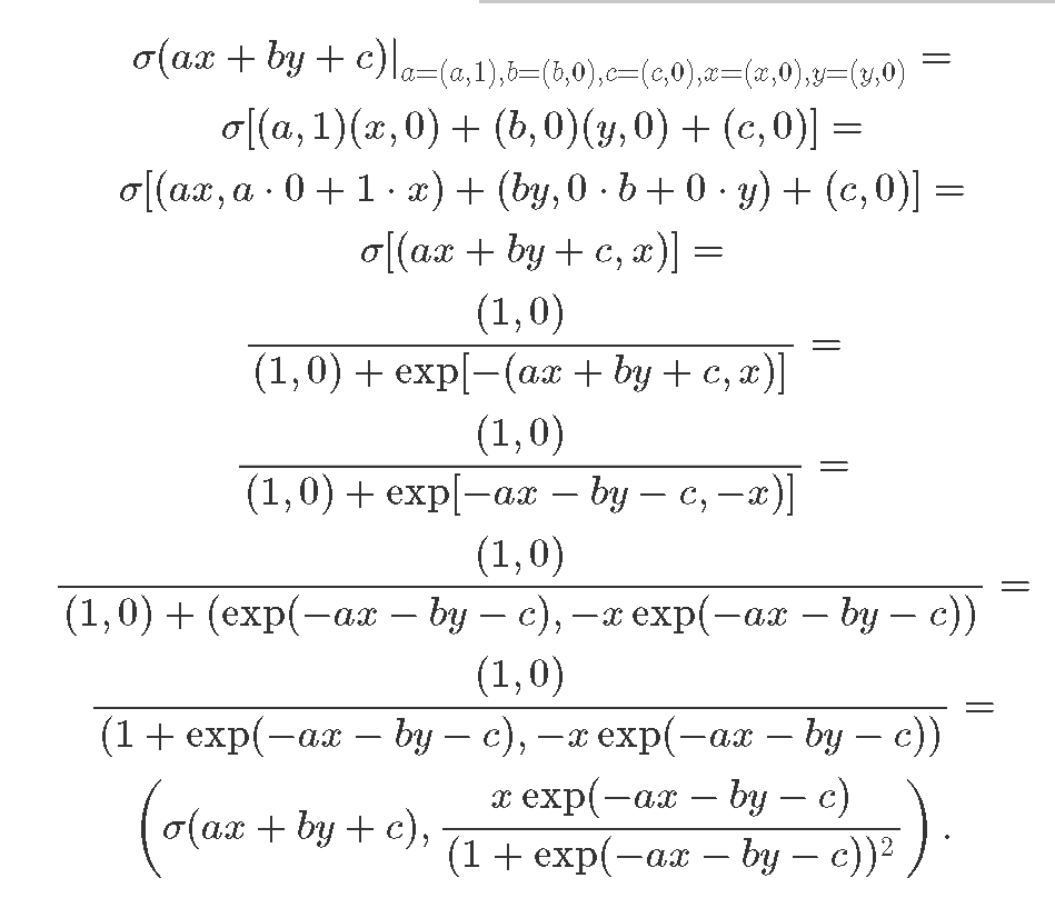The first expression is the result of neuron's computation and the second one is the exact analytic expression for

. That is all the magic behind automatic differentiation! In a similar way, we can obtain the rest of the gradients:

neuron1 [(1, 0), (2, 1), (-3, 0), (-1, 0), (3, 0)]
(0.8807970779778823,0.3149807562105195)

neuron1 [(1, 0), (2, 0), (-3, 1), (-1, 0), (3, 0)]
(0.8807970779778823,0.1049935854035065)

neuron1 [(1, 0), (2, 0), (-3, 0), (-1, 1), (3, 0)]
(0.8807970779778823,0.1049935854035065)

neuron1 [(1, 0), (2, 0), (-3, 0), (-1, 0), (3, 1)]
(0.8807970779778823,0.209987170807013)

Introducing backprop library

The backprop library was specifically designed for differentiable programming. It provides combinators to reduce our mental overhead. In addition, the most useful operations such as arithmetics and trigonometry, have already been defined in the library. See also hmatrix-backprop for linear algebra. So all you need for differentiable programming now is to define some functions:

neuron
  :: Reifies s W
  => [BVar s Double] -> BVar s Double
neuron [a, b, c, x, y] = sigmoid (a * x + b * y + c)

sigmoid x = 1 / (1 + exp (-x))

Here BVar s wrapper signifies that our function is differentiable. Now, the forward pass is:

forwardNeuron = BP.evalBP (neuron. BP.sequenceVar)

We use sequenceVar isomorphism to convert a BVar of a list into a list of BVars, as required by our neuron equation. And the backward pass is

backwardNeuron = BP.gradBP (neuron. BP.sequenceVar)

abcxy0 :: [Double]
abcxy0 = [1, 2, (-3), (-1), 3]

forwardNeuron abcxy0
-- 0.8807970779778823

backwardNeuron abcxy0
-- [-0.1049935854035065,0.3149807562105195,0.1049935854035065,0.1049935854035065,0.209987170807013]

Note that all the gradients are in one list, the type of the first neuron argument.

Summary

Modern neural networks tend to be complex beasts. Writing backpropagation gradients by hand can easily become a tedious task. In this post we have seen how automatic differentiation can face this problem.

In the next posts we will apply automatic differentiation to real neural networks. We will talk about batch normalization, another crucial method in modern deep learning. And we will ramp it up to convolutional networks allowing us to solve some interesting challenges. Stay tuned!