День 4: Важность пакетной нормализации

WhichДля purposeкакой doцели neuralсуществуют networksнейронные serveсети? for?Нейронные Neuralсети networks- areэто learnableобучаемые models.модели. TheirИх ultimateглавная goalцель is- toприблизиться approachили orдаже evenпревзойти surpassчеловеческие humanспособности cognitiveвосприятия. abilities.Ричард AsСуттон Richardговорит, Suttonчто putsсамый it,большой 'Theуро, biggestкоторый lessonможет thatбыть canполучен be read fromс 70 yearsгодов ofразработки AIИИ, researchв isтом, thatчто generalобщие methodsметоды thatиспользующие leverageвычисления computationочень are ultimately the most effective'эффективны. InВ hisего essay,эссе, SuttonСуттон arguesговорит, thatчто onlyтолько modelsмодели withoutбез encodedзашифрованного human-knowledgeчеловеческого canзнания outperformмогут human-centericпревзойти approaches.человеко-ориентированные Indeed,подходы. neuralТак, networksчто areнейронные generalсети enoughв andобщем theyбудут leverageдостаточны computation.для Then,использования itвычислений. isЗатем, notне surprisingудивительно, howчто theyони canмогут exhibitвыставить millionsмиллионы ofобучаемых learnableстепеней degrees of freedom.свободы.

TheСамый biggestбольшой challengeвызов withдля neuralнейронных networksсетей: is two-fold: (1) howкак toобучить trainэти thoseмиллионы millionsпараметров, of parameters, and (2) howкак toих interpretинтерпритировать. them.Пакетная Batch normalization нормализация(shortly batchnorm) wasбыл introducedпредставлен asв anкачестве attemptпопытки toсделать makeобучение trainingеще moreэффективнее. efficient.Метод Theможет methodсильно canсократить dramaticallyчисло reduceитераций theобучения. numberДаже of training epochs. Moreover,больше, batchnorm is- perhapsвозможо theявляется keyключем, ingredientкоторый thatдаст madeвозможность possibleобучать trainingопределенные ofархитектуры certainтакие architecturesкак suchбинарная asнейронная binarizedсеть. neural networks. Finally,Наконец, batchnorm isодна oneиз ofсамых theпоследних mostпреимуществ recentнейронной neural network advances1.сети.

PreviousПакетная postsнормализация в кратце

DayЧто 1:такие Learningпакет? NeuralДо Networksсих Theпор, Hardвы Wayсмотрели Dayна 2:игрущечные Whatнаборы Doданных. HiddenОни Layersбыли Do?настолько Dayмалы, 3:что Haskellмогли Guideбыть Toлегко Neuralпомещены Networksв Theпамять. sourceОднако, codeв fromреальности thisсуществует postогромные isнаборы availableзанимающие onсотни Github.гигабайтов памяти, такие как Imagenet. Они часто не помещаются в память. В этом случае, имеет смысл разделить наборы данных в маленькие пакеты. Во время обучения обрабатывается только один пакет.

BatchКак Normalizationпредполагает In Short What Is A Batch? Until now, we have looked on toy datasets. These were so small that they could completely fit into the memory. However, in the real world exist huge databases occupying hundreds of gigabytes of memory, such as Imagenet for example. Those often would not fit into the memory. In that case, it makes more sense to split a dataset into smaller mini-batches. During a forward/backward pass, only one batch is typically processed.

As the name suggests,имя, batchnorm transformationпреобразование isэто actingдействие onнад individualотдельными batchesпакетами of data. The outputs of linear layers may cause activation function saturation/'dead neurons'данных. ForВывод instance,линейного inслоя caseможет ofбыть причиной деградации активационной функции. Например: в случае ReLU (rectified linear unit) f(x)=max(0,x) activation,активация, allвсе negativeнегативные valuesзначения willбудут resultприводить inк zeroнулевой activations.активации. Therefore,Отсюда, itхорошая isидея a- goodнормализовать ideaэти toзначения normalizeс thoseпомощью valuesвычитания by subtracting the batch meanсреднего μ пакета. Similarly,Похожим divisionобразом, byделение standardпо deviationстандартному отклоненю √var scalesмасштабирует theамплитуту, amplitudes,которая whichособенно isвыгодня especiallyдля beneficialактивация forсигмоидного sigmoid-like activations.вида.

TrainingОбучение Andи Batchnorm

TheПроцеедура batchпакетной normalizationнормализации procedureимеет differsотличия betweenна theэтапах trainingобучения andи inferenceвывода. phases.Во Duringвремя theобучения, training,каждый forслой, eachгде layerмы whereхотим weприменить wantbatchnorm, toсначала applyвычисляем batchnormсредний weмини first compute the mini-batch mean:пакет:

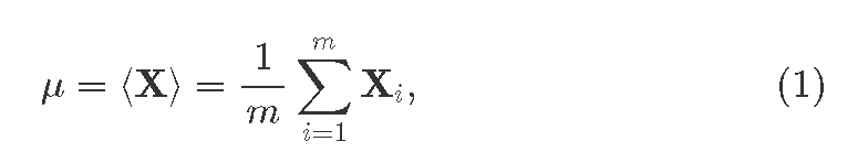
whereгде Xi is theэто i thвектор-свойство feature-vectorидущий comingиз fromпрошлого the previous layer;слоя; i=1…m, whereгде m>1 isэто theразмер batchпакета. size.Так Weже alsoполучаем obtainди:сперсию theдля mini-batch variance:пакета

Now,

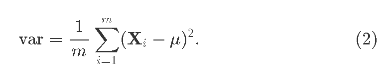
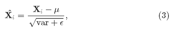
Теперь thebatchnorm batchnorm'sядро, heart,сама normalization itself:нормализация: whereгде aмаленькая small constantпостоянная ϵ isдобавляет addedчисловую forстабильность. numericalЧто stability.если Whatнормализация ifданного normalizationслоя ofбыла theвредна? givenАлгоритм layerпредоставит wasдва harmful?обучаемых Theпараметра, algorithmкоторые providesв twoхудшем learnableслучае parametersмогут thatотменить inэффект theпакетной worstнормализации: caseсмасштабирует scenario can undo the effect of batch normalization: scaling parameterпараметр γ andи shiftувеличит β. 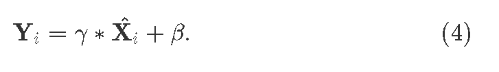AfterПосле (optionally)применения applyingтаковых those,мы weполучим obtainвывод theслоя output of the batchnorm layer:batchnorm: PleaseОтметим, noteчто thatоба: bothсреднее meanзначениее μ andи varianceраспределение var areвекторы vectorsколичество ofкоторых asтакое manyже elementsбольшое asкак neuronsи inнейронов aв givenданном hiddenскрытом layer.слое. OperatorОператор ∗ denotesговорит element-wiseо multiplication.поэлементном умножении.

InferenceВывод

InВ theстадии inferenceвывода phaseлучше itвсего isиметь perfectlyодну normalвыборку toданных haveза oneраз. dataКак sampleже atсосчитать aсреднюю time.величину Soпакета howесли toцелый calculateпакет batchэто meanи ifесть theвыборка wholeданных? batchДля isправильной aобраотки, singleво sample?время Toобучения properlyмы handleуказываем this,среднее duringзначение trainingи we estimate mean and varianceраспределение (E[X] and Var[X]) overдля allвсех trainingнаборов set.обучения. ThoseЭти vectorsвектора will replaceзаменят μandиvar` duringво inference,время avoidingвывода, thusтаким theобразом problemизбегая ofпроблемы normalizingнормализации aединичного singleton batch.пакета.

HowНасколько Efficient Isэффективен Batchnorm

So far we have played with tasks that provided low-dimensional input features. Now, we are going to test neural networks on a bit more interesting challenge. We will apply our skills to automatically recognize human-written digits on a famous MNIST dataset. This challenge came from the need to have zip-code machine reading for more efficient postal services.

We construct two neural networks, each having two fully-connected hidden layers (300 and 50 neurons). Both networks receive 28×28=784 inputs, the number of image pixels, and give back 10 outputs, the number of recognized classes (digits). As in-between layer activations we apply ReLU f(x)=max(0,x). To obtain the classification probabilities vector in the result, we use softmax activation . One of the networks in addition performs batch normalization before ReLUs. Then, we train those using stochastic gradient descent2 with learning rate α=0.01^3 and batch size m=100.

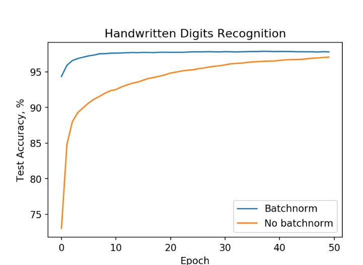
Neural network training on MNIST data. Training with batchnorm (blue) leads to high accuracies faster than without batchnorm (orange).

From the figure above we see that the neural network with batch normalization reaches about 98 % accuracy in ten epochs, whereas the other one is struggling to reach comparable performance in fifty epochs! Similar results can be obtained for other architectures.

It is worth mentioning that we still may lack understanding how exactly does batchnorm help. In its original paper, it was hypothesized that batchnorm is reducing internal covariate shift. Recently, it was shown that that is not necessary true. The best up-to-date explanation is that batchnorm makes optimization landscape smooth, thus making gradient descent training more efficient. This, in its turn, allows using higher learning rates than without batchnorm!

Implementing batchnorm

We will base our effort on the code previously introduced on Day 2. First, we will redefined the Layer data structure making it more granular:

data Layer a = -- Linear layer with weights and biases
               Linear (Matrix a) (Vector a)
               -- Same as Linear, but without biases
               | Linear' (Matrix a)
               -- Batchnorm with running mean, variance, and two
               -- learnable affine parameters
               | Batchnorm1d (Vector a) (Vector a) (Vector a) (Vector a)
               -- Usually non-linear element-wise activation
               | Activation FActivation

Amazing! Now we can distinguish between several kinds of layers: affine (linear), activation, and batchnorm. Since batchnorm already compensates for a bias, we do not actually need biases in the subsequent linear layers. That is why we define a Linear' layer without biases. We also extend Gradients to accommodate our new layers structure:

data Gradients a = -- Weight and bias gradients
                   LinearGradients (Matrix a) (Vector a)
                   -- Weight gradients
                   | Linear'Gradients (Matrix a)
                   -- Batchnorm parameters and gradients
                   | BN1 (Vector a) (Vector a) (Vector a) (Vector a)
                   -- No learnable parameters
                   | NoGrad

Next, we want to extend the neural network propagation function _pass, depending on the layer. That is easy with pattern matching. Here is how we match the Batchnorm1d layer and its parameters:

    _pass inp (Batchnorm1d mu variance gamma beta:layers)
        = (dX, pred, BN1 batchMu batchVariance dGamma dBeta:t)
      where

As previously, the _pass function receives an input inp and layer parameters. The second argument is the pattern we are matching against, making our algorithm specific in this case for (Batchnorm1D ...). We will also specify _pass for other kinds of Layer. Thus, we have obtained a polymorphic _passfunction with respect to the layers. Finally, the equation results in a tuple of three: gradients to back propagatedX, predictions pred, and prepended list twith valuesBN1computed in this layer (batch meanbatchMu, variance batchVariance`, and learnable parameters gradients).

The forward pass as illustrated in this post:

        -- Forward
        eps = 1e-12
        b = br (rows inp)  -- Broadcast (replicate) rows from 1 to batch size
        m = recip $ (fromIntegral $ rows inp)

        -- Step 1: mean from Equation (1)
        batchMu :: Vector Float
        batchMu = compute $ m `_scale` (_sumRows inp)

        -- Step 2: mean subtraction
        xmu :: Matrix Float
        xmu = compute $ inp .- b batchMu

        -- Step 3
        sq = compute $ xmu .^ 2

        -- Step 4: variance, Equation (2)
        batchVariance :: Vector Float
        batchVariance = compute $ m `_scale` (_sumRows sq)

        -- Step 5
        sqrtvar = sqrtA $ batchVariance `addC` eps

        -- Step 6
        ivar = compute $ A.map recip sqrtvar

        -- Step 7: normalize, Equation (3)
        xhat = xmu .* b ivar

        -- Step 8: rescale
        gammax = b gamma .* xhat

        -- Step 9: translate, Equation (4)
        out0 :: Matrix Float
        out0 = compute $ gammax .+ b beta

As discussed on Day 2, there is a recurrent call obtaining gradients from the next layer, neural network prediction pred and computed values tail t:

        (dZ, pred, t) = _pass out layers

I prefer to keep the backward pass without any simplifications. That makes clear which step corresponds to which:

        -- Backward

        -- Step 9
        dBeta = compute $ _sumRows dZ

        -- Step 8
        dGamma = compute $ _sumRows (compute $ dZ .* xhat)
        dxhat :: Matrix Float
        dxhat = compute $ dZ .* b gamma

        -- Step 7
        divar = _sumRows $ compute $ dxhat .* xmu
        dxmu1 = dxhat .* b ivar

        -- Step 6
        dsqrtvar = (A.map (negate. recip) (sqrtvar .^ 2)) .* divar

        -- Step 5
        dvar = 0.5 `_scale` ivar .* dsqrtvar

        -- Step 4
        dsq = compute $ m `_scale` dvar

        -- Step 3
        dxmu2 = 2 `_scale` xmu .* b dsq

        -- Step 2
        dx1 = compute $ dxmu1 .+ dxmu2
        dmu = A.map negate $ _sumRows dx1

        -- Step 1
        dx2 = b $ compute (m `_scale` dmu)

        dX = compute $ dx1 .+ dx2

Note that often we need to perform operations like mean subtraction X−μ, where in practice we have a matrix X and a vector μ. How do you subtract a vector from a matrix? Right, you don't. You can subtract only two matrices. Libraries like Numpy may have a broadcasting magic that would implicitly convert a vector to a matrix5. This broadcasting might be useful, but might also obscure different kinds of bugs. We instead perform explicit vector to matrix transformations. For our convenience, we have a shortcut b = br (rows inp) that will expand a vector to the same number of rows as in inp. Where function br ('broadcast') is:

br rows' v = expandWithin Dim2 rows' const v

Here is an example how br works. First, we start an interactive Haskell session and load NeuralNetwork.hs module:

$ stack exec ghci
GHCi, version 8.2.2: http://www.haskell.org/ghc/  :? for help
Prelude> :l src/NeuralNetwork.hs

Then, we test br function on a vector [1, 2, 3, 4]:

*NeuralNetwork> let a = A.fromList Par [1,2,3,4] :: Vector Float
*NeuralNetwork> a
Array U Par (Sz1 4)
  [ 1.0, 2.0, 3.0, 4.0 ]

*NeuralNetwork> let b = br 3 a
*NeuralNetwork> b
Array D Seq (Sz (3 :. 4))
  [ [ 1.0, 2.0, 3.0, 4.0 ]
  , [ 1.0, 2.0, 3.0, 4.0 ]
  , [ 1.0, 2.0, 3.0, 4.0 ]
  ]

As we can see, a new matrix with three identical rows has been obtained. Note that a has type Array U Seq, meaning that data are stored in an unboxed array. Whereas the result is of type Array D Seq, a so-called delayed array. This delayed array is not an actual array, but rather a promise to compute6 an array in the future. In order to obtain an actual array residing in memory, use compute:

*NeuralNetwork> compute b :: Matrix Float
Array U Seq (Sz (3 :. 4))
  [ [ 1.0, 2.0, 3.0, 4.0 ]
  , [ 1.0, 2.0, 3.0, 4.0 ]
  , [ 1.0, 2.0, 3.0, 4.0 ]
  ]

You will find more information about manipulating arrays in massiv documentation. Similarly to br, there exist several more convenience functions, rowsLike and colsLike. Those are useful in conjunction with _sumRows and _sumCols:

-- | Sum values in each column and produce a delayed 1D Array
_sumRows :: Matrix Float -> Array D Ix1 Float
_sumRows = A.foldlWithin Dim2 (+) 0.0

-- | Sum values in each row and produce a delayed 1D Array
_sumCols :: Matrix Float -> Array D Ix1 Float
_sumCols = A.foldlWithin Dim1 (+) 0.0

Here is an example of _sumCols and colsLike when computing softmax activation

softmax :: Matrix Float -> Matrix Float
softmax x =
  let x0 = compute $ expA x :: Matrix Float
      x1 = compute $ (_sumCols x0) :: Vector Float
      x2 = x1 `colsLike` x
  in (compute $ x0 ./ x2)

Note that softmax is different from element-wise activations. Instead, softmax acts as a fully-connected layer that receives a vector and outputs a vector. Finally, we define our neural network with two hidden linear layers and batch normalization as:

  let net = [ Linear' w1
            , Batchnorm1d (zeros h1) (ones h1) (ones h1) (zeros h1)
            , Activation Relu
            , Linear' w2
            , Batchnorm1d (zeros h2) (ones h2) (ones h2) (zeros h2)
            , Activation Relu
            , Linear' w3
            ]
```haskell
The number of inputs is the total number of `28×28=784`
 image pixels and the number of outputs is the number of classes (ten digits). We randomly generate the initial weights `w1`, `w2`, and `w3`. And set initial batchnorm layer parameters as follows: means to zeroes, variances to ones, scaling parameters to ones, and translation parameters to zeroes:
```haskell
  let [i, h1, h2, o] = [784, 300, 50, 10]
  (w1, b1) <- genWeights (i, h1)
  let ones n = A.replicate Par (Sz1 n) 1 :: Vector Float
      zeros n = A.replicate Par (Sz1 n) 0 :: Vector Float
  (w2, b2) <- genWeights (h1, h2)
  (w3, b3) <- genWeights (h2, o)

Remember that the number of batchnorm parameters equals to the number of neurons. It is a common practice to put batch normalization before activations, however this sequence is not strict: one can put batch normalization after activations too. For comparison, we also specify a neural network with two hidden layers without batch normalization.

  let net2 = [ Linear w1 b1
             , Activation Relu
             , Linear w2 b2
             , Activation Relu
             , Linear w3 b3
             ]

In both cases the output softmax activation is omitted as it is computed together with loss gradients in the final recursive call in _pass:

    _pass inp [] = (loss', pred, [])
      where
        pred = softmax inp
        loss' = compute $ pred .- tgt

Here, [] on the left-hand side signifies an empty list of input layers, and [] on the right-hand side is the empty tail of computed values in the beginning of the backward pass.

The complete project is available on Github. I recommend playing with different neuron networks architectures and parameters. Have fun!

Batchnorm Pitfalls

There are several potential traps when using batchnorm. First, batchnorm is different during training and during inference. That makes your implementation more complicated. Second, batchnorm may fail when training data come from different datasets. To avoid the second pitfall, it is essential to ensure that every batch represents the whole dataset, i.e. it has data coming from the same distribution as the machine learning task you are trying to solve. Read more about that.

Summary

Despite its pitfalls, batchnorm is an important concept and remains a popular method in the context of deep neural networks. Batchnorm's power is that it can substantially reduce the number of training epochs or even help achieving better neural network accuracy. After discussing this, we are prepared for such hot subjects as convolutional neural networks and reinforcement learning. Stay tuned!

AI And Neural Networks

• Richard Sutton. The Bitter Lesson
• Using neural nets to recognize handwritten digits
• Batch normalization paper
• How Does Batch Normalization Help Optimization?
• On The Perils of Batch Norm

Haskell

• Why I think Haskell is the best general purpose language
• An opinionated beginner's guide to Haskell in mid 2019
• Massiv Array Library
• Alexey's presentation about massiv