День 4: Важность пакетной нормализации

Для какой цели существуют нейронные сети? Нейронные сети - это обучаемые модели. Их главная цель - приблизиться или даже превзойти человеческие способности восприятия. Ричард Суттон говорит, что самый большой уро, который может быть получен с 70 годов разработки ИИ, в том, что общие методы использующие вычисления очень эффективны. В его эссе, Суттон говорит, что только модели без зашифрованного человеческого знания могут превзойти человеко-ориентированные подходы. Так, что нейронные сети в общем будут достаточны для использования вычислений. Затем, не удивительно, что они могут выставить миллионы обучаемых степеней свободы.

Самый большой вызов для нейронных сетей: 1) как обучить эти миллионы параметров, 2) как их интерпритировать. Пакетная нормализация(batchnorm) был представлен в качестве попытки сделать обучение еще эффективнее. Метод может сильно сократить число итераций обучения. Даже больше, batchnorm - возможо является ключем, который даст возможность обучать определенные архитектуры такие как бинарная нейронная сеть. Наконец, batchnorm одна из самых последних преимуществ нейронной сети.

Пакетная нормализация в кратце

Что такие пакет? До сих пор, вы смотрели на игрущечные наборы данных. Они были настолько малы, что могли быть легко помещены в память. Однако, в реальности существует огромные наборы занимающие сотни гигабайтов памяти, такие как Imagenet. Они часто не помещаются в память. В этом случае, имеет смысл разделить наборы данных в маленькие пакеты. Во время обучения обрабатывается только один пакет.

Как предполагает имя, batchnorm преобразование это действие над отдельными пакетами данных. Вывод линейного слоя может быть причиной деградации активационной функции. Например: в случае ReLU f(x)=max(0,x) активация, все негативные значения будут приводить к нулевой активации. Отсюда, хорошая идея - нормализовать эти значения с помощью вычитания среднего μ пакета. Похожим образом, деление по стандартному отклоненю √var масштабирует амплитуту, которая особенно выгодня для активация сигмоидного вида.

Обучение и Batchnorm

Процеедура пакетной нормализации имеет отличия на этапах обучения и вывода. Во время обучения, каждый слой, где мы хотим применить batchnorm, сначала вычисляем средний мини пакет:

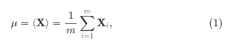где Xi это i вектор-свойство идущий из прошлого слоя; i=1…m, где m>1 это размер пакета. Так же получаем ди:сперсию для пакета

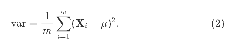
Теперь batchnorm ядро, сама нормализация: 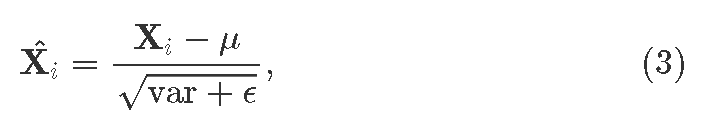где маленькая постоянная ϵ добавляет числовую стабильность. Что если нормализация данного слоя была вредна? Алгоритм предоставит два обучаемых параметра, которые в худшем случае могут отменить эффект пакетной нормализации: смасштабирует параметр γ и увеличит β. После применения таковых мы получим вывод слоя batchnorm: 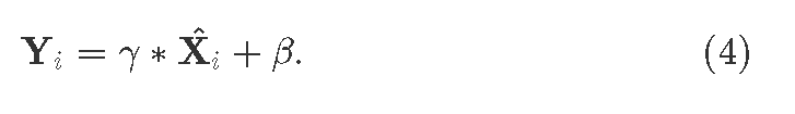Отметим, что оба: среднее значениее μ и распределение var векторы количество которых такое же большое как и нейронов в данном скрытом слое. Оператор ∗ говорит о поэлементном умножении.

Вывод

В стадии вывода лучше всего иметь одну выборку данных за раз. Как же сосчитать среднюю величину пакета если целый пакет это и есть выборка данных? Для правильной обраотки, во время обучения мы указываем среднее значение и распределение (E[X] and Var[X]) для всех наборов обучения. Эти вектора заменят μиvar` во время вывода, таким образом избегая проблемы нормализации единичного пакета.

Насколько эффективен Batchnorm

So far we have played with tasks that provided low-dimensional input features. Now, we are going to test neural networks on a bit more interesting challenge. We will apply our skills to automatically recognize human-written digits on a famous MNIST dataset. This challenge came from the need to have zip-code machine reading for more efficient postal services.

We construct two neural networks, each having two fully-connected hidden layers (300 and 50 neurons). Both networks receive 28×28=784 inputs, the number of image pixels, and give back 10 outputs, the number of recognized classes (digits). As in-between layer activations we apply ReLU f(x)=max(0,x). To obtain the classification probabilities vector in the result, we use softmax activation 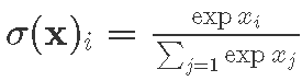. One of the networks in addition performs batch normalization before ReLUs. Then, we train those using stochastic gradient descent2 with learning rate α=0.01^3 and batch size m=100.

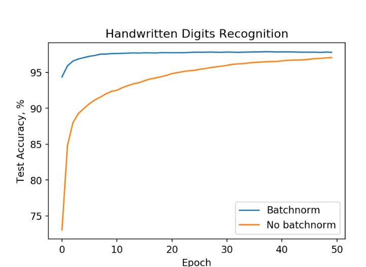
Neural network training on MNIST data. Training with batchnorm (blue) leads to high accuracies faster than without batchnorm (orange).

From the figure above we see that the neural network with batch normalization reaches about 98 % accuracy in ten epochs, whereas the other one is struggling to reach comparable performance in fifty epochs! Similar results can be obtained for other architectures.

It is worth mentioning that we still may lack understanding how exactly does batchnorm help. In its original paper, it was hypothesized that batchnorm is reducing internal covariate shift. Recently, it was shown that that is not necessary true. The best up-to-date explanation is that batchnorm makes optimization landscape smooth, thus making gradient descent training more efficient. This, in its turn, allows using higher learning rates than without batchnorm!

Implementing batchnorm

We will base our effort on the code previously introduced on Day 2. First, we will redefined the Layer data structure making it more granular:

data Layer a = -- Linear layer with weights and biases
               Linear (Matrix a) (Vector a)
               -- Same as Linear, but without biases
               | Linear' (Matrix a)
               -- Batchnorm with running mean, variance, and two
               -- learnable affine parameters
               | Batchnorm1d (Vector a) (Vector a) (Vector a) (Vector a)
               -- Usually non-linear element-wise activation
               | Activation FActivation

Amazing! Now we can distinguish between several kinds of layers: affine (linear), activation, and batchnorm. Since batchnorm already compensates for a bias, we do not actually need biases in the subsequent linear layers. That is why we define a Linear' layer without biases. We also extend Gradients to accommodate our new layers structure:

data Gradients a = -- Weight and bias gradients
                   LinearGradients (Matrix a) (Vector a)
                   -- Weight gradients
                   | Linear'Gradients (Matrix a)
                   -- Batchnorm parameters and gradients
                   | BN1 (Vector a) (Vector a) (Vector a) (Vector a)
                   -- No learnable parameters
                   | NoGrad

Next, we want to extend the neural network propagation function _pass, depending on the layer. That is easy with pattern matching. Here is how we match the Batchnorm1d layer and its parameters:

    _pass inp (Batchnorm1d mu variance gamma beta:layers)
        = (dX, pred, BN1 batchMu batchVariance dGamma dBeta:t)
      where

As previously, the _pass function receives an input inp and layer parameters. The second argument is the pattern we are matching against, making our algorithm specific in this case for (Batchnorm1D ...). We will also specify _pass for other kinds of Layer. Thus, we have obtained a polymorphic _passfunction with respect to the layers. Finally, the equation results in a tuple of three: gradients to back propagatedX, predictions pred, and prepended list twith valuesBN1computed in this layer (batch meanbatchMu, variance batchVariance`, and learnable parameters gradients).

The forward pass as illustrated in this post:

        -- Forward
        eps = 1e-12
        b = br (rows inp)  -- Broadcast (replicate) rows from 1 to batch size
        m = recip $ (fromIntegral $ rows inp)

        -- Step 1: mean from Equation (1)
        batchMu :: Vector Float
        batchMu = compute $ m `_scale` (_sumRows inp)

        -- Step 2: mean subtraction
        xmu :: Matrix Float
        xmu = compute $ inp .- b batchMu

        -- Step 3
        sq = compute $ xmu .^ 2

        -- Step 4: variance, Equation (2)
        batchVariance :: Vector Float
        batchVariance = compute $ m `_scale` (_sumRows sq)

        -- Step 5
        sqrtvar = sqrtA $ batchVariance `addC` eps

        -- Step 6
        ivar = compute $ A.map recip sqrtvar

        -- Step 7: normalize, Equation (3)
        xhat = xmu .* b ivar

        -- Step 8: rescale
        gammax = b gamma .* xhat

        -- Step 9: translate, Equation (4)
        out0 :: Matrix Float
        out0 = compute $ gammax .+ b beta

As discussed on Day 2, there is a recurrent call obtaining gradients from the next layer, neural network prediction pred and computed values tail t:

        (dZ, pred, t) = _pass out layers

I prefer to keep the backward pass without any simplifications. That makes clear which step corresponds to which:

        -- Backward

        -- Step 9
        dBeta = compute $ _sumRows dZ

        -- Step 8
        dGamma = compute $ _sumRows (compute $ dZ .* xhat)
        dxhat :: Matrix Float
        dxhat = compute $ dZ .* b gamma

        -- Step 7
        divar = _sumRows $ compute $ dxhat .* xmu
        dxmu1 = dxhat .* b ivar

        -- Step 6
        dsqrtvar = (A.map (negate. recip) (sqrtvar .^ 2)) .* divar

        -- Step 5
        dvar = 0.5 `_scale` ivar .* dsqrtvar

        -- Step 4
        dsq = compute $ m `_scale` dvar

        -- Step 3
        dxmu2 = 2 `_scale` xmu .* b dsq

        -- Step 2
        dx1 = compute $ dxmu1 .+ dxmu2
        dmu = A.map negate $ _sumRows dx1

        -- Step 1
        dx2 = b $ compute (m `_scale` dmu)

        dX = compute $ dx1 .+ dx2

Note that often we need to perform operations like mean subtraction X−μ, where in practice we have a matrix X and a vector μ. How do you subtract a vector from a matrix? Right, you don't. You can subtract only two matrices. Libraries like Numpy may have a broadcasting magic that would implicitly convert a vector to a matrix5. This broadcasting might be useful, but might also obscure different kinds of bugs. We instead perform explicit vector to matrix transformations. For our convenience, we have a shortcut b = br (rows inp) that will expand a vector to the same number of rows as in inp. Where function br ('broadcast') is:

br rows' v = expandWithin Dim2 rows' const v

Here is an example how br works. First, we start an interactive Haskell session and load NeuralNetwork.hs module:

$ stack exec ghci
GHCi, version 8.2.2: http://www.haskell.org/ghc/  :? for help
Prelude> :l src/NeuralNetwork.hs

Then, we test br function on a vector [1, 2, 3, 4]:

*NeuralNetwork> let a = A.fromList Par [1,2,3,4] :: Vector Float
*NeuralNetwork> a
Array U Par (Sz1 4)
  [ 1.0, 2.0, 3.0, 4.0 ]

*NeuralNetwork> let b = br 3 a
*NeuralNetwork> b
Array D Seq (Sz (3 :. 4))
  [ [ 1.0, 2.0, 3.0, 4.0 ]
  , [ 1.0, 2.0, 3.0, 4.0 ]
  , [ 1.0, 2.0, 3.0, 4.0 ]
  ]

As we can see, a new matrix with three identical rows has been obtained. Note that a has type Array U Seq, meaning that data are stored in an unboxed array. Whereas the result is of type Array D Seq, a so-called delayed array. This delayed array is not an actual array, but rather a promise to compute6 an array in the future. In order to obtain an actual array residing in memory, use compute:

*NeuralNetwork> compute b :: Matrix Float
Array U Seq (Sz (3 :. 4))
  [ [ 1.0, 2.0, 3.0, 4.0 ]
  , [ 1.0, 2.0, 3.0, 4.0 ]
  , [ 1.0, 2.0, 3.0, 4.0 ]
  ]

You will find more information about manipulating arrays in massiv documentation. Similarly to br, there exist several more convenience functions, rowsLike and colsLike. Those are useful in conjunction with _sumRows and _sumCols:

-- | Sum values in each column and produce a delayed 1D Array
_sumRows :: Matrix Float -> Array D Ix1 Float
_sumRows = A.foldlWithin Dim2 (+) 0.0

-- | Sum values in each row and produce a delayed 1D Array
_sumCols :: Matrix Float -> Array D Ix1 Float
_sumCols = A.foldlWithin Dim1 (+) 0.0

Here is an example of _sumCols and colsLike when computing softmax activation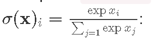

softmax :: Matrix Float -> Matrix Float
softmax x =
  let x0 = compute $ expA x :: Matrix Float
      x1 = compute $ (_sumCols x0) :: Vector Float
      x2 = x1 `colsLike` x
  in (compute $ x0 ./ x2)

Note that softmax is different from element-wise activations. Instead, softmax acts as a fully-connected layer that receives a vector and outputs a vector. Finally, we define our neural network with two hidden linear layers and batch normalization as:

  let net = [ Linear' w1
            , Batchnorm1d (zeros h1) (ones h1) (ones h1) (zeros h1)
            , Activation Relu
            , Linear' w2
            , Batchnorm1d (zeros h2) (ones h2) (ones h2) (zeros h2)
            , Activation Relu
            , Linear' w3
            ]
```haskell
The number of inputs is the total number of `28×28=784`
 image pixels and the number of outputs is the number of classes (ten digits). We randomly generate the initial weights `w1`, `w2`, and `w3`. And set initial batchnorm layer parameters as follows: means to zeroes, variances to ones, scaling parameters to ones, and translation parameters to zeroes:
```haskell
  let [i, h1, h2, o] = [784, 300, 50, 10]
  (w1, b1) <- genWeights (i, h1)
  let ones n = A.replicate Par (Sz1 n) 1 :: Vector Float
      zeros n = A.replicate Par (Sz1 n) 0 :: Vector Float
  (w2, b2) <- genWeights (h1, h2)
  (w3, b3) <- genWeights (h2, o)

Remember that the number of batchnorm parameters equals to the number of neurons. It is a common practice to put batch normalization before activations, however this sequence is not strict: one can put batch normalization after activations too. For comparison, we also specify a neural network with two hidden layers without batch normalization.

  let net2 = [ Linear w1 b1
             , Activation Relu
             , Linear w2 b2
             , Activation Relu
             , Linear w3 b3
             ]

In both cases the output softmax activation is omitted as it is computed together with loss gradients in the final recursive call in _pass:

    _pass inp [] = (loss', pred, [])
      where
        pred = softmax inp
        loss' = compute $ pred .- tgt

Here, [] on the left-hand side signifies an empty list of input layers, and [] on the right-hand side is the empty tail of computed values in the beginning of the backward pass.

The complete project is available on Github. I recommend playing with different neuron networks architectures and parameters. Have fun!

Batchnorm Pitfalls

There are several potential traps when using batchnorm. First, batchnorm is different during training and during inference. That makes your implementation more complicated. Second, batchnorm may fail when training data come from different datasets. To avoid the second pitfall, it is essential to ensure that every batch represents the whole dataset, i.e. it has data coming from the same distribution as the machine learning task you are trying to solve. Read more about that.

Summary

Despite its pitfalls, batchnorm is an important concept and remains a popular method in the context of deep neural networks. Batchnorm's power is that it can substantially reduce the number of training epochs or even help achieving better neural network accuracy. After discussing this, we are prepared for such hot subjects as convolutional neural networks and reinforcement learning. Stay tuned!