MONDAY MORNING HASKELL

• Отрыв
• Haskell 101: Установка, Выражения, Типы
• Модули и синтаксис функций
• Делая свой тип.
• Мозги Haskell
• Часть 1: Ослабим страшный взгляд Haskell
• Часть 2: Обучение обучению
• Часть 3: Haskell и взвешенная практика
• Часть 4: Обучение управляемое компиляцией
• Монады (и другие функциональные структуры)
• Функторы
• Аппликативные функторы
• Монады
• Монады Reader и Writer
• State Монада
• Преобразователи Монад
• Законы Монад
• Testing in Haskell
• TDD и базовые библиотеки
• Profiling and Benchmarking
• Improving Performance with Data Structures
• Haskell's Data Types!
• PART 1: HASKELL'S SIMPLE DATA TYPES
• Sum Types in Haskell
• Parameterized Types in Haskell
• Haskell Typeclasses as Inheritance
• Type Families in Haskell
• Real World Haskell
• Databases and Persistent
• Building an API with Servant!
• Redis Caching
• Testing with Docker
• Esqueleto and Complex Queries
• Machine Learning in Haskell
• Haskell and Tensor Flow
• Haskell, AI, and Dependent Types I
• Haskell, AI, and Dependent Types II
• Grenade and Deep Learning
• Haskell & Open AI Gym
• Open AI Gym Primer: Frozen Lake
• Frozen Lake in Haskell
• Open AI Gym: Blackjack
• Basic Q-Learning
• Generalizing Our Environments
• Q-Learning with TensorFlow (Haskell)
• Rendering with Gloss
• Parsing with Haskell
• Parsing Primer: Gherkin Syntax
• Applicative Parsing
• Attoparsec
• Megaparsec
• Haskell API Integrations
• Twilio and Text Messages
• Sending Emails with Mailgun
• Mailchimp and Building Our Own Integration
• Contributing to GHC
• Contributing to GHC 1: Preparation
• Contributing to GHC 2: Basic Hacking and Organization
• Contributing to GHC 3: Hacking Syntax and Parsing
• Elm: Functional Frontend
• Elm Part 1: Language Basics
• Elm Part 2: Making a Single Page App
• Elm Part 3: Adding Effects
• Elm Part 4: Navigation
• Purescript: Haskell + Javascript
• Purescript Part 1: Basics of Purescript
• Purescript Part 2: Typeclasses and Monads
• Purescript Part 3: Simple Web UI's
• Purescript Part 4: Web Requests and Navigation

Отрыв

Haskell 101: Установка, Выражения, Типы

Добро пожаловать в первую часть серии Отрыва Понедельнечного Хаскельного Утра! Если вы мечтали попробовать изучить Haskell,но никогда не могли найти хорошее руководство для этого, вы в правильном месте! У вас может не быть знания об этом прекрасном языке. Но после прочтения трех статей, вы должны будете знать базовые идеи достаточно, чтобы начать программировать самостоятельно.

Эта статья покрывает несколько различных тем. Первая, мы скачаем всё необходимое и установи. Затем мы начнем писать наше первое выражение и изучим немного про систему типов в Haskell. Дальше, мы поместим "функцию" в функциональное программирование и изучик что Haskell функции являются объектом первого класса. Наконец, мы затронем тему более сложных типов таких как списки и кортежи.

Если вы уже читали эту стать или знакомы со всеми этими концептами, вы можете перепрыгнуть ко второй части. В ней мы поговорим о написании своих фалов с кодаи и написании более сложных функций с некоторым дополнительным синтаксом. Обязательно загляните в главу 3, где мы посмотрим на то, как легко создавать свой собственный тип данных!

Эта серия, так же, с примерами в репозитории Github. Этот репозиторий позволит вам работать с некоторыми примерами кода из этих статей. В этой первой части, мы в основном будет работать с GHCI, нежели с файлами.

Наконец, как только вы закончите с этим, проверьте себя с помощью чеклиста. Это даст вам возможность проверить свои знания со всех сторон.

Установка

Если вы еще не касались Haskell совем, первый шаг - скачать платформу Haskell. Скачаем последнюю версию для вашей ОС и проследуем по подсказкам на экране.

Платфрма содержит 4 главных сущности. Первая - GHC, широко распространненый компилятор Haskell. Компилятор это то, что превращает код в что-то что компьютер может запустить. Второе - GHCI, интерпретатор для языка Haskell. Он позволяет вам вводить выражения и тестировать некоторые вычисления без того, чтоб использовать отдельный файл.

Третье - Cabal, менеджер зависимости для Haskell библиотек. Он позволяет вам скачивать код, который другие люди уже написали и используют в своих проектах. Наконец, инструмент Stack. Он добавляет еще один слой поверх Cabal и делает его проще для скачивания пакетов, с которыми не хотелось бы иметь конфликтов. Если хотите более детальное рассмотрение этой темы, можно взглянуть на Stack Mini-Course!

Чтобы проверить. что у вас все работает правильно, нужно запустить команду ghci в вашем терминале и дождаться запуска интепретатора. Мы проведем остаток этой лекции в GHCI пытая некоторые базовые свойства языка.

Выражения

У вас уже все установленно, давайте пойдем дальше! Самое фундаментальное в Haskell - всё что пишется это выражение. Все программы состоят из вычисления этих выражений. Давайте начнем с проверки некоторых, самых простых выражений, которые мы можем сделать. Веедите следующее выражение в интерпретатор. Каждый раз при нажатии enter, интерпретатор должен просто выводить обратно то, что вы ввели.

>> True
True
>> False
False
>> 5
5
>> 5.5
5.5
>> 'a'
'a'
>> "Hello"
"Hello

Этим набором выражений, мы покрыли большую часть базовых типов языка. Если вы делали программы ранее, эти базовые типы должны быть вам хорошо знакомы. Первыве два выражения - булевы. True и False - единственные значения этого типа. Мы так же можем делать выражения из чисел, целых и десятичных. Наконец, мы можем делать выражения отображающием отдельные символы так же как и целые слова, которые мы назовем string.

В интерпретаторе, мы можем назначить выражения для наименования используя let и знак равно. Это сохранит выражение под именем к которому мы можем ссылаться позже.

>> let firstString = "Hello"
>> firstString
"Hello"

Тип

Теперь, одно из классных вещей о Haskell это то, что любое выражение имеет тип. Давайте проверим тип базового выражения которое мы ввели вышее. Мы увидим, что идея о которой мы говорим формализованна и самом языке. Вы можете посмотреть тип любого выражения используя команду :t commang.

>> :t True
True :: Bool
>> :t False
False :: Bool
>> :t 5
5 :: Num t => t
>> :t 5.5
5.5 :: Fractional t => t
>> :t 'a'
'a' :: Char
>> :t "Hello"
"Hello" :: [Char]

Пара выражений проста, но другая пара кажется странной. Последнее выражение это же просто строка? Верно. Вы можете использовать понятие String в вашем коде. Но под капотом, Haskell думает о строках как о списке символов, о чем говорит [Char]. Мы вернемся к этому позже. True и False отвечает за тип Bool, как мы и ожидаем. Символ a просто единичный Char. Наши числа немного сложнее. Временно игнорируем слова Num и Fractional. Это то как мы можем ссылаться на различные типы. Мы будем представлять себе целые числа в качестве Int типа, а с плавающей запятой как Double. Мы можем явно назначить тип:

>> let a = 5 :: Int
>> :t a
a :: Int
>> let b = 5.5 :: Double
>> :t b
b :: Double

Мы уже можем увидеть, что-то очень интересно о Haskell. Он может взаимодействовать с информацией о типе нашего выражения просто исходя из формы. В общем, нам не нужно явно давать тип для каждого нашего выражения как мы делали в языках Java или С++.

Функции

Давайте начнем делать некоторые вычисления с нашими выражениями и увидим, что будет происходить. Мы можем начать с которых базовых математических вычислений:

>> 4 + 5
9
>> 10 - 6
4
>> 3 * 5
15
>> 3.3 * 4
13.2
>> (3.3 :: Double) * (4 :: Int)

В то время, как мы закончили с этой частью, мы поняли что здесь происходит и как мы можем это исправить. Теперь, важная заметка, всё в Haskell - выражение, и любое выржаение имеет свой тип. Логично, мы должны уметь узнавать и определять типа этих различных выражений. И мы определенно можем это делать. Нам нужно просто обернуть в скобки. чтобы убедиться, что тип команды знал, что нужно включить выражение целиком.

>> let a = 4 :: Int
>> let b = 5 :: Int
>> a + b
9
>> :t (a + b)
(a + b) :: Int

Оператор +, даже сам по себе без числе, всё еще выражение! Это наш первй пример функции, или выражения которое принимает аргументы. Когда мы обращаемся к нему самому то его нужно обернуть в скобки.

>> :t (+)
(+) :: Num a => a -> a -> a

Это наш первый пример отражения типа функции. Важная часть тут - a -> a -> a. Это выражение говорит нам что (+) это функция которая принимает два аргумента, которые дожны иметь один и тот же ти. И затем выдает нам результат того же типа, что и входные данные. Num указывает, что нам нужно использовать числовые типы, вроде целых и с плавающей запятой. Мы не можем например сделать так:

>> "Hello " + "World"

Но есть объяснение тому, почему нельзя сложить напрмер Int и Double вместе. Функция требует использовать одинаковый тип для обоих аргументов. Чтобы это исправить, нам нужно использовать другую функци для того. чтобы изменить тип одного из аргумента, чтобы он совпадал с другим. Или мы можем позволить взаимодействию типов разрешить это самому, как мы делали это в примере выше. Но мы бежим вперед поезда. Давайте остановимся на смысле того как мы "применяем" эти функции.

В общем, мы "применяем" функции помещая аргумент после функции. Фнукция (+) специальная, так как мы можем использовать её между аргументами. Если мы всё таки хотим, то можем использовать скобки вокруг нее и поставим как обычную функцию вначале. В этом случае оба аргумента будут и стоять после.

>> (+) 4 5
9

Что важно знать про функции, то что не обязательно использовать сразу все аргументы. Мы можем взять тот же оператор сложения и применит только одно число. Это называется частичное применние.

>> let a = 4 :: Int
>> :t (a +)
(a +) :: Int -> Int

Сам по себе (+) оператор которы принимает 2 аргумента. Сейчас мы к нему применили один аргумент, который принимает оставшийся. Дальше, так как один аргумент был Int второй тоже должен быть Int. Мы можем использовать частичное применение для выражения используя let и затем применить второй аргумент.

>> let f = (4 +)
>> f 5
9

Давайте немного поэкспериментируем с другими операторами, в этот раз с булевым типом. Это очень важно, потому, что они позволят создавать более сложные условия когда начнете писать функции. Это три главных оператора, которые работают таким образом, как вы ожидаете для других языков: And, Or и Not. Первые два принимают два булевых параметра и возвращают один, последний принимает одно значение и возвращает одно.

>> :t (&&)
(&&) :: Bool -> Bool -> Bool
>> :t (||)
(||) :: Bool -> Bool -> Bool
>> :t not
not :: Bool -> Bool

Ну и взглянем на простые примеры поведения:

>> True && False
False
>> True && True
True
>> False || True
True
>> not True
False

Последнюю функцию которую мы разберем - функция равенства. Принимает два аргумента почти любого типа и определяет равны ли они или нет.

>> 5 == 5
True
>> 4.3 == 4.8
False
>> True == False
False
>> "Hello" == "Hello"
True

Списки

Теперь мы собираемся слегка расширить наши горизонты и обсудить еще больше типов. Первая идея на которую взглянем это список. Это последовательность значений, которые имеют один тип. Определяется список с помощью квадратных скобочек. Список может не иметь элементов совсем, и такой пустой список можно вызывать.

>> :t [1,2,3,4,7]
[1,2,3,4,7] :: Num t -> [t]
>> :t [True, False, True]
[True, False, True] :: [Bool]
>> :t ["Hello", True]
Error! (these aren't the same type!)
>> :t []
[] :: [t]

Отметим ошибку в третьем примере! Списки не могут иметь различныне типы элементов. Помните, мы говорили ранее, что строка это просто список симолов. Теперь посмотрим как выглядит строка:

>> "Hello" == ['H', 'e', 'l', 'l', 'o']
True

Списки можно объединить используя оператор (++). Так как строки - списки, это позволяет нам комбинировать строки как в любом другом языке.

>> [1,2,3] ++ [4,5,6]
[1,2,3,4,5,6]
>> "Hello " ++ "World"
"Hello World"

Списки так же имеют две функции, которые специально спроектированны, что получения определенных элементов. Мы можем использовать head функцияю, что получения первого элемента списки. И похожим образом, мы можемт использовать tail функцию для получения всех элементов, кроме первого(head).

>> head [1,2,3]
1
>> tail [True, False, False]
[False, False]
>> tail [3]
[]

Внимание! Вызов обоих функции для пустого списка приведет к ошибке!

>> head []
Error!
>> tail []
Error!

Кортежи

Теперь мы знаем о списках, вы можете гадать, если есть способ объединять элементы которые не имеют одинаковый тип. На самом деле есть! Называются они Кортежи! Можно создать кортеж, который будет иметь любое количество элементов, который со своим типом. Кортежи обозначаются с помощью круглых скобок.

>> :t (1 :: Int, "Hello", True)
(1 :: Int, "Hello", True) :: (Int, [Char], Bool)
>> :t (1 :: Int, 2 :: Int)
(1 :: Int, 2 :: Int) :: (Int, Int)

Каждый кортеж, котоый мы делаем имеет свой собственный тип основываясь на типах элементов внутри кортежа. Это значит, что следующие любые типы, даже если элементы будут иметь одинаковый тип, или иметь одинаковую длинну.

>> :t (1 :: Int, 2 :: Int)
(1 :: Int, 2 :: Int) :: (Int, Int)
>> :t (2 :: Int, 3 :: Int, 4 :: Int)
(2 :: Int, 3 :: Int, 4 :: Int) :: (Int, Int, Int)
>> :t ("Hi", "Bye", "Good")
([Char], [Char], [Char])

Так как кортежи это выражения, как и другие, мы можем его выводить! Однако, мы не можемт объединять кортежи различных типов в один список.

>> :t [(1 :: Int, 2 :: Int), (3 :: Int, 4 :: Int)]
[(1 :: Int, 2 :: Int), (3 :: Int, 4 :: Int)] :: [(Int, Int)]
>> :t [(True, False, True), (False, False, False)]
[(Bool, Bool, Bool)]
>> :t [(1,2), (1,2,3)]
Error

Заключение

Конец первой части нашей отрывной серии. Взгляните на то, что мы прошли в одной статье. Мы установили Haskell платформу и начали экспериментировать с GHCI, интерпретатором кода. Мы так же узнали о выражениях, типах, функциях которые являются строительными элементами Haskell.

Во второй части этого набора, мы начнем писать наш код на Haskell в исходных файлах и изучим еще синтаксис языка. Проверим как мы можемт вывести что-то пользователю из нашей программы, и как можно получить что-то от пользователя на вход. Так же начнем писать наши функции и посмотрим на различные способы для указания поведения функций.

В третьей части, мы начнем создавать свой тип данных. Мы посмотрим насколько просты алгебраические типы данных Haskell, и как типы synonym и newtypes может дать нам дополнительное управление через кодовый стиль.

Модули и синтаксис функций

Вновь, добро пожаловать на серию Отрыв Понедельнечного Хаскельного Утра! Это вторая часть серии. Если вы пропустили первую часть, то вам стоит вернуться к ней, где вы сможете скачать, устаноить все необходимое. Мы так же пройдем через базовые идеи выражений, типов и функций.

Теперь вы возможно думаете: "Изучение типов с помощью интерпритатора - весело! Но я хочу писать настоящий код!" На что поход Haskell синтакс? К счастью, на этом мы и сосредоточимся.

Мы наченм писать наш модуль и функции. Посмотрим на то, как читать наш код в интерпретаторе и как запустить его через испольнительный файл. Еще изучим подробнее синтакс функйий для описания более сложных идей. В части третьей этой серии, мы узнаем, как создать свой тип данных!

Если вы хотите проследовать вместе с примерами кода в этойй части, вы можете пройти в репозиторий на Github и скачать. Ссылки будут указаны дальше в статье.

Написание файлов с исходным кодом

Теперь, вы знакомы с базовыми идеями Haskell, мы должны начать писать наш код. Для этой первой части статьи, вы скачать исходинк с Github. Или вы можете написать самостоятельно. Давайте наченм с открытия файла под названием MyFirstModule.hs, и объявим в нем Haskell модуль используя ключевое слово module в самом верху файла.

module MyFirstModule where

Выражение where следует за именем модуля и отражает начальную точку нашего кода. Давайте напишем очень простое выржаение, которое наш модуль будет экспортировать. На назначим выражению имя используя знак равно. В отличии от интерпретатора, нам не нужно использовать слово let.

myFirstExpression = "Hello World!"

Когда определяется выражение внутри модуля, распространенная практика это указать его сигнатуту в самом верхнем уровне выражения и функции. Это важно понять для любого кто собирается читать ваш код. Это так же помогает компилятору выводит типы внутри вашего подвыражений. Давайте пойдем дальше, и пометим выражение используя в качестве String используя оператор ::.

myFirstExpression :: String
myFirstExpression = "Hello World!"

Так же определим нашу первую функцию. Она будет принимать String в качестве ввода, и складывать входную строку со строкой "Hello". Отметим, как мы определим тип функции используя стрелку от входного типа в выходной.

myFirstFunction :: String -> String
myFirstFunction input = "Hello " ++ input

Теперь имея этот код, мы можем загрузить наш модуль в GHCi. Чтобы сделать это запустим GHCi из той же директории где лежит модуль. Вы можеет использовать :load команду для загрузки всех опеределений выражений, чтобы и меть доступ к ним. Давайте посмотрим на это в действии:

>> :load MyFirstModule
(loaded)
>> myFirstExpression
"Hello World!"
>> myFirstFunction "Friend"
"Hello Friend"

Если мы изменили наш исходный код, мы можем вернуться обратно и перезагрузить модуль в GHCi используя :r команду("reload"). Давайте изменим функции как показано ниже:

myFirstFunction :: String -> String
myFirstFunction input = "Hello " ++ input ++ "!"

Теперь перезагрузим и запустим еще раз!

>> :r
(reloaded)
>> myFirstFunction "Friend"
"Hello Friend!"

Ввод и вывод.

В конце, мы хотим иметь возможность запускать наш код без нужны использовать интерпретатор. Чтобы это сделать мы превратим наш модуль в бинарный файл. Делается это с помощью добавления функции под названием main со специальной сигнатурой.

main :: IO ()

Этот и сигнатуры может казаться странным, так как мы еще не говорили ни о каком IO или () пока. Всё что вам нужно понять, то что этот тип сигнатуры позволяет нашей main функции взаимодействовать с терминалом. Мы можем, например, запустить некоторые выражение вывода. Для этого воспользуемся специальным синтаксом называемым "do-syntax". Будем использовать слово do, и затем перечислим возможные действия вывода на каждой линии под.

main :: IO ()
main = do
  putStrLn "Running Main!"
  putStrLn "How Exciting!"

Теперь у нас есть эта главная функция, нам не нужно использовать интерпретатор. Мы можем использовать терминальную команду runghc.

> runghc ./MyFirstModule
Running Main!
How Exciting!

Конечно, вы так же можете хотет иметь возможность читать ввод от пользователя, и вызывать различные функции. Для этого нужно воспользоваться функцией getLine. Вы можете получить доступ используя специальный оператор <-. Затем с помощью "do-syntax", можно будет использовать let как делали в интерпретаторе для назначения выражению имени. В этом случае мы вызовем наше прошлое выражение.

main :: IO ()
main = do
  putStrLn "Enter Your Name!"
  name <- getLine
  let message = myFirstFunction name
  putStrLn message

Попробуем запустить.

> runghc ./MyFirstModule.hs
Enter Your Name!
Alex
Hello Alex!

Вот так, мы написали нашу первую маленькую Haskell программу.

IF и ELSE синтакс

Теперь мы собираемся немного подвинуться, и посмотреть на то как мы можем сделать нашу функцию более интересной используя Haskell синтакс конструктор. Есть две возможности для этого. Вы можете ссылаться на полный файл который имеет весь конечный код, который мы пишем в этой части. Или вы можете использовать метод "сделай сам", где придется самостоятельно заполнить определения как показано в статье.

Первая синтаксическая идея которую мы изучем будет выражение if. Давайте предполжим, мы хотим попросить пользовтаеля ввести число. Затем вы делаем различные действия в зависимости от того насколько большое число.

Выражение if немного отличается в Haskell от того, к чему мы привыкли. Для примера, следующее выражение легко понимается в Java:

if (a <= 2) {
  a = 4;
}

Такие выражения не могут существовать в Haskell! Все выражения if должны иметь else ветвление! Чтобы понять почему, нам нужно вернуться к основам из прошлой статьи. Помните, все в Haskell это выражение, и любое выражение имеет тип. Так как мы можемт назначить выражению имя, что оно будет значить для имени если выражение станет false? Давайте взглянем на пример правильного if выражения:

myIfStatement a = if a <= 2
  then a + 2
  else a - 2

Это законченное выражение. На первой лини, мы написали выражения типа Bool, которое может выдать True или False. На второй строке, мы написали выражение, которое будет результатом если результат будет True. Третья строка сработает если результат проверки будет False.

Помните, любое выражение имеет тип. Так каков же тип этого if выражения? Предпололжим наш ввод имеет тип Int. В этом случае, обе ветви тоже будут Int, значит тип нашего выражения должен быть тоже Int.

Remember every expression has a type. So what is the type of this if-expression? Suppose our input is an Int. In this case, both the branches (a+2 and a - 2) are also ints, so the type of our expression must be an Int itself.

myIfStatement :: Int -> Int
myIfStatement a = if a <= 2
  then a + 2
  else a - 2

Что случиться, если мы попробуем сделать, так, что строки будут иметь различный тип?

myIfStatement :: Int -> ???
myIfStatement a = if a <= 2
  then a + 2
  else "Hello"

Результатом будет ошибка, не важно какой бы тип мы не пытались указать в качестве результат. Это важный урок для выражения if. У вас есть две ветви, и каждая ветвь должна выдавать тот же результат. Результирующий тип это тип всего выражения.

Отступление, наш пример будет вести к тому, чтобы вы использовали определенный вид записи. Однако, вы можете собрать всё в одной строке.

myIfStatement :: Int -> Int
myIfStatement a = if a <= 2 then a + 2 else a - 2

В Haskell нет elif выражения как в Puthon. Но подобный механизм достижим. Вы можете использовать if выражение как целое выражение для ветви else.

myIfStatement :: Int -> Int
myIfStatement a = if a <= 2
  then a + 2
  else if a <= 6
    then a
    else a - 2

Охранные выражения(GUARDS)

В случаее когда мы хотите обработать различные ситуации, для читабельности кода в нем можно использовать охранные выражения. Охранные выражения позволяют вам проверять любое число различных условий. Мы можем переписать код выше используя их.

myGuardStatement :: Int -> Int
myGuardStatement a
  | a <= 2 = a + 2
  | a <= 6 = a
  | otherwise = a - 2

Есть пара тонкостей. Первая - нам не нжно использовать ключевое слово else с охранными выражениями, используется otherwise. Второе - каждый отдельный случай имеет свой собственный = знак, и это не = знак для всего выражения. Ваш код не соберется если вы попробуете написать, что-то подобное:

myGuardStatement :: Int -> Int
myGuardStatement a = -- BAD!
  | a <= 2 ...
  | a <= 6 ...
  | otherwise = ...

Сопоставление с образцом.

В отличии от других языков, Haskell имеет другой способ ветвления в коде кроме булевых типов. Вы можете так же произвести сопоставление с образом(pattern matching). Это позволит изменить поведение кода основываясь на структуре объекта. Для примера, мы можем написать множество версий функции каждя из которых работает на определенном виде аргументов. Вот пример, который ведет себя по другому основывась на типе списка, который он получает.

myPatternFunction :: [Int] -> Int
myPatternFunction [a] = a + 3
myPatternFunction [a,b] = a + b + 1
myPatternFunction (1 : 2 : _) = 3
myPatternFunction (3 : 4 : _) = 7
myPatternFunction xs = length xs

Первый пример будет совпадать с любым списком который содержит отдельный элемент. Второй пример будет совпадать с любыми примером у которого два элемента. Третий пример использует некоторый синтакс объединения с которым мы еще не знакомы. Но он совпадает с любым списком который начинается с элемента 1 или 2. Следующая строка, любой список, который начинается с 3 и 4. Последний пример будет совпадать с другими списками.

Важно отметить, каким способо шаблоны связывают значения с именами. В первом примере, один элемент списка связан с именем, так, что мы можем использовать его в выражении. В последнем примере, полный список связан с xs, поэтому мы можем использовать его в выражении, чтобы мы могли взять его длинну. Давайте посмотрим на эти примеры в действии.

>> myPatternFunction [3]
6
>> myPatternFunction [1,2]
4
>> myPatternFunction [1,2,8,9]
3
>> myPatternFunction [3,4,1,2]
7
>> myPatternFunction [2,3,4,5,6]
5

Порядок выражений важен! Второй пример имеет такие же шаблоны (1 : 2 : _). Но так как мы сначала указали [1,2] шаблон, он будет использовать эту версию функции. Если мы поставим универсальное значение первым, то всегда будет выполняться только этот универсальный шаблон.

-- BAD! Function will always return 1!
myPatternFunction :: [Int] -> Int
myPatternFunction xs = 1
myPatternFunction [a] = a + 3
myPatternFunction [a,b] = a + b + 1
myPatternFunction (1 : 2 : _) = 3
myPatternFunction (3 : 4 : _) = 7

К счастью, компилятор предупредит нас о том, что мы не используем какие шаблоны сопоставления с образцом.

>> :load MyFirstModule
MyFirstModule.hs:31:1: warning: [-Woverlapping-patterns]
Pattern match is redundant
In an equation for ‘myPatternFunction': myPatternFunction [a] = ...

MyFirstModule.hs:32:1: warning: [-Woverlapping-patterns]
Pattern match is redundant
In an equation for ‘myPatternFunction': myPatternFunction [a, b] = ...

MyFirstModule.hs:33:1: warning: [-Woverlapping-patterns]
Pattern match is redundant
In an equation for ‘myPatternFunction': myPatternFunction (1 : 2 : _) = ...

MyFirstModule.hs:34:1: warning: [-Woverlapping-patterns]
Pattern match is redundant
In an equation for ‘myPatternFunction': myPatternFunction (3 : 4 : _) = ...

Последним хочется отметить, нижнее подчеркивание(как показано выш) может быть использованно для любого шаблона, который мы не хотим использовать. Это универсальная функция и работает для любого значения.

myPatternFunction _ = 1

Условные выражения

Вы можете использовать сопоставление с образом в середине функции и условными выражениями. Можно переписать прошлый пример так:

myCaseFunction :: [Int] -> Int
myCaseFunction xs = case xs of
  [a] -> a + 3
  [a,b] -> a + b + 1
  (1 : 2 : _) -> 3
  (3 : 4 : _) -> 7
  xs -> length xs

Отметим, что мы используем стрелку -> вместо знака равно для каждого случая. Условные выражения более обобщены, проще использовать внутри функции. Для примера:

myCaseFunction :: Bool -> [Int] -> Int
myCaseFunction usePattern xs = if not usePattern
  then length xs
  else case xs of
    [a] -> a + 3
    [a,b] -> a + b + 1
    (1 : 2 : _) -> 3
    (3 : 4 : _) -> 7
    _ -> 1

WHERE и LET

Если вы пришли из императивного языка, вы должно быть наблюдаете сейчас. И отметили, что похоже мы никогда не объявляем промежуточные переменные. Все выражения, что используются, получаются из шаблонов аргументов. Haskell не имет технически переменных, так как выражения не меняют их значения!Но все еще можем изменить подвыражение внутри нашей функции. Есть пара различных способов для этого. Давайте представим один приме, где мы производим несколько математических операций на входе.

mathFunction :: Int -> Int -> Int -> Int
mathFunction a b c = (c - a) + (b - a) + (a * b * c) + a

Пока мы можем поздравить друг друга с тем, что функция написана в строку, этот код не совсем читаем. Мы можем сделать его более читаемым используя промежуточные выражения. Для начала сделаем это используя where выражение.

mathFunctionWhere :: Int -> Int -> Int -> Int
mathFunctionWhere a b c = diff1 + diff2 + prod + a
  where
    diff1 = c - a
    diff2 = b - a
    prod = a * b * c

Часть where объявляет diff1, diff2 и diff3 в качестве промежуточоного значения. Потом мы можем использовать их в качестве базы функции. Мы можем использовать where результаты друг с другом, и не важно в каком порядке они объявленны.

mathFunctionWhere :: Int -> Int -> Int -> Int
mathFunctionWhere a b c = diff1 + diff2 + prod + a
  where
    prod = diff2 * b * c
    diff1 = c - a
    diff2 = b - diff1

Однако, нужно быть уверенным в том, что вы не делаете цикл where, где каждый результат завит от соседнего.

mathFunctionWhere :: Int -> Int -> Int -> Int
mathFunctionWhere a b c = diff1 + diff2 + prod + a
  where
    diff1 = c - diff2
    diff2 = b - diff1 -- BAD! This will cause an infinite loop!
                      --      diff1 depends on diff2!
    prod = a * b * c

Мы можем получить тот же результат используя let выражение. Синтаксически похожая формулировка, за исключением нового выражения перед. Нам потом, нужно использовать ключевое слово для указания выражеения которое будет использовать значения.

mathFunctionLet :: Int -> Int -> Int -> Int
mathFunctionLet a b c =
  let diff1 = c - a
      diff2 = b - a
      prod = a * b * c
  in diff1 + diff2 + prod + a

В ситуации с IO как мы писали вывод и чтения, можно использовать let в качестве действия без требования. Вам просто нужно сделать это без использования where когда ваше выражение зависит от пользовательского ввода.

main :: IO ()
main = do
  input <- getLine
  let repeated = replicate 3 input
  print repeated

Мы можем обойти эту тему. Мы можем использовать where для объявления функции внутри нашей функции. Пример выше можно переписать по другому:

main :: IO ()
main = do
  input <- getLine
  print (repeatFunction input)
  where
    repeatFunction xs = replicate 3 xs

В этом примере, мы объявили repeatFunction как функцию, котораяа принимает список(или String в нашем случае). Зтаем на строке print, мы передаем входную строку в качестве аргумента в функциюю. Класс!

Заключение

Мы изучили очень много всего! Начали с написания нашего кода, получение ввода, выведения в терминал, и запуска нашего прилоежния в качестве исполнительного файла. Изучили расширенный синтакс функции. Изучили if-выражения, сопоставление с образом, выражения where и let.

Если вас что-то смутило, не бойетсь, вернитесь и проверьте еще раз первую статью, для того, чтобы устаканить ваши знания в типа выражений! Если вам всё понятно - двигайтесь дальше к следующей статье. В ней мы обсудим различные способы создания нашего собственного типа данных в Haskell.

Делая свой тип.

Вновь, добро пожаловать на серию Отрыв Понедельнечного Хаскельного Утра! Заключительная часть. На случай, если вы прпоустили 2 прошлые главы. В первой части мы обсудили базовую установку Haskell платформы. Затем окунулись в написание базовых выражений на Haskell в интерпретаторе. Во второй части, мы начали с написания нашей собственной функции в модуле Haskell. Так же изучили всяких синтаксических уловок для построения больших и улучшенных функций.

В третьей части мы собираемся углубиться в системы типов. Изучим как создавать свои типы данных, а так же хитрости для упрощения описания наших типов.

Созание нового типа данных

Вперед, к типам данных! Помните, что у нас есть github репозиторий где вы можете получить код для этой части. Если вы хотите реализовать его самостоятельно, вы можете перейти к модулю DataTypes. Но если вы просто хотите посмотреть на завершенный код, вы можете взглянут на DataTypesComplete.

Для этой статьи, предскавим. что мы пытаемся смоделировать некий TODO список. В этой статье создадим несколько различных Task типов данных для отражения отдельных задач в списке. Создадим тип данных сначала у которого будет ключевое слово и затем имя типа. Затем добавим оператор присваивания =.

module DataTypes where

data Task1 = ...

В отличии от выражения и функции именя которые мы использовали в ранее, наши типы начинаются с заглавной буквы. Это то что отличает типы от обычных выражений в Haskell. Теперь собираемся создать наш первый конструктор. Это специальный тип выражения, который позволяет нам создавать объект нашего типа Task. Они имеют схожесть с конструкторами скажем на Java. Но они они так же очень сложны. Конструкторы имеют Заглавные буквы а так же список типов. Этот список типов содержит информацию которую хранит конструктор. В нашем случае, мы хотим, чтобы наша задача имела имя и ожидаемоее время выполнения в минутах, отражены как String, и Int соответственно.

data Task1 = BasicTask1 String Int

Вот так, теперь мы можем начать создавать Task объекты. Например, давайте определим пару простых задач как выражения в нашем модуле.

assignment1 :: Task1
assignment1 = BasicTask1 "Do assignment 1" 60

laundry1 :: Task1
laundry1 = BasicTask1 "Do Laundry" 45

Мы можем загрузить наш код в интерпретатор, чтоы проверить что он собирается и имеет смысл:

>> :l MyData.hs
>> :t assignment1
assignment1 :: Task1
>> :t laundry1 
laundry1 :: Task

Отметим, что тип нашего выражения Task1 даже не смотря, что мы собираемся объекты используя BasicTask1Constructor. В Java, можно иметь множество конструкторов для одного типа. Мы можем сделать так же и в Haskell, но выглядит это по сложнее. Давайте определим другой тип для различных мест, где мы можем работать над задачами. Мы можем производить работу над задачами в школе, офисе, дома. Отразим это создава конструктор для каждого из них. Разделим конструктор используя вертикальную черту |:

data Location =
  School |
  Office |
  Home

В этом случае, каждый из конструкторов простая отметка, которая не имеет параметров или данных хранящихся в нем. Это пример Enum типа. Мы можем технически сделать различные типы выражения отражающими каждый из них.

schoolLocation :: Location
schoolLocation = School

officeLocation :: Location
officeLocation = Office

homeLocation :: Location
homeLocation = Home

Но эти выражения не более полезны чем использовать сами конструкторы.

Теперь, имея пару типов, мы можем сделать так, что один из наших типов будет содержать другие! Добавим новый конструктор в наш тип задач. Это будет еще сложнее чем просто список мест.

data Task1 =
  BasicTask1 String Int |
  ComplexTask1 String Int Location
...

complexTask :: Task1
complexTask = ComplexTask1 "Write Memo" 30 Office

Это сильно отличается от конструктора в других языках. Мы можем иметь различные поля для различных отображений типов. Можно обернуть совершенно отличающийся тип зависящий от конструктора который мы используем. Это отлично, так как дает нам гибкость, которую ругие языке не могут.

Параметризированные типы

Еще использовать параметризированные типы с другими определениями типов. Это значит, что один или более полей зависят от типа, который был выбран человеком который писал код. Давайте предположим, у нас есть тип, который имеет несколько базовых конструкторов для различных видов времени. Это ограничит наше описание для простоты.

data TaskLength =
  QuarterHour |
  HalfHour |
  ThreeQuarterHour |
  Hour |
  HourAndHalf |
  TwoHours |
  ThreeHours

Теперь мы хотим описать задачу где время задачи будет выражатся в Int. Но так же хотим, чтобы была возможность описать с помощью нового типа. Давайте сделаем вторую верси нашего Task типа, который может использовать оба типа для времени выполнения. Мы можем сделать это с помощью параметризованного типа:

data Task2 a =
  BasicTask2 String a |
  ComplexTask2 String a Location

Тип стал мистическим, и теперь мы можем его заполнять как хотим. Но теперь при выводе Task2 типа в сигнатуре, мы должны будет заполнить правильное определение.

assignment2 :: Task2 Int
assignment2 = BasicTask2 "Do assignment 2" 60

assignment2' :: Task2 TaskLength
assignment2' = BasicTask2 "Do assignment 2" Hour

laundry2 :: Task2 Int
laundry2 = BasicTask2 "Do Laundry" 45

laundry2' :: Task2 TaskLength
laundry2' = BasicTask "Do Laundry" ThreeQuarterHour

complexTask2 :: Task2 TaskLength
complexTask2 = ComplexTask2 "Write Memo" HalfHour Office

К этом нужно относится с осторожностью, так как это может ограничить нашу возможность делать определнные вещи. Например, мы не можем создать список, который содержит оба и assignment2 и complexTask2. Это потому, что два выражения теперь различные типы.

-- THIS WILL CAUSE A COMPILER ERROR
badTaskList :: [Task2 a]
badTaskList = [assignment2, complexTask2]

Пример списка

Говоря о списках, мы можем приоткрыть завесу тайны о том, как списки реализованны.

Большое количество синтаксического сахара меняют способ написания списка на практике. Но на уровне кода, списки определяются двумя конструкторами, Nil и Cons.

data List a =
  Nil |
  Cons a (List a)

Как мы ожидаем, тип List имеет один параметр. Это то что позволяет нам одновременно иметь Int или String. Конструктор Nil это пустой список. Не содержит объектов. Поэтому в любое время, в которое вы будете использовать выражение [], занайте вы используете Nil. Второй конструктор складывает один элемент с другим списком. Тип элемента и списка должны, конечно же совпадать. При использовании : оператора для добавления элемента в список, вы уже используете Cons конструктор.

emptyList :: [Int]
emptyList = [] -- Actually Nil

fullList :: [Int]
-- Equivalent to Cons 1 (Cons 2 (Cons 3 Nil))
-- More commonly written as [1,2,3]
fullList = 1 : 2 : 3 : []

Еще одна вещь, то что наша структура данных рекурсивна. Мы можем увидеть в Cons конструкторе как список содержит другой список с параметрами. Это Работает отлично, покоа есть какой-то базовый случай! Тогда, у нас будет Nil. Представьте если у нас есть один конструктор и он принимает рекурсивный параметр. У нас возникает затруднительное положение, из-за того, что мы не знаем как создать любойс писок на первом месте.

Синтаксическая записи

Давайте вернемся к основам, непараметризированному типу данных Task. Предположим, нас не волнует в целом объект Task. Скорее, мы хотим один из его кусочков, напиример имя или время. Так как наш код - единственный способ сделать это использовать сопоставление с образцом который явит нужное поле.

import Data.Char (toUpper)

...

twiceLength :: Task1 -> Int
twiceLength (BasicTask1 name time) = 2 * time

capitalizedName :: Task1 -> String
capitalizedName (BasicTask1 name time) = map toUpper name

tripleTaskLength :: Task1 -> Task1
tripleTaskLength (BasicTask1 name time) = BasicTask1 name (3 * time)

Теперь слегка упрощаем. Вы можете использовать нижнее подчеркивание вместо параметра, который вы не хотите исопльзовать. Но несмотря на это, может получится громоздко если у ваш тип имеет ножество полей. Мы можем написать нашу функцию позволяющую иметь доступ к отдельным полям. Под капотом, конечно же, будет сопоставление с образом.

taskName :: Task1 -> String
taskName (BasicTask1 name _) = name

taskLength :: Task1 -> Int
taskLength (BasicTask1 _ time) = time

twiceLength :: Task1 -> Int
twiceLength task = 2 * (taskLength task)

capitalizedName :: Task1 -> String
capitalizedName task = map toUpper (taskName task)

tripleTaskLength :: Task1 -> Task1
tripleTaskLength task = BasicTask1 (taskName task) (3 * (taskLength task))

Но это применение нельзя масштабировать, так как нам нужно писать эту функцию для каждого поля, которое мы будем создавать. Теперь представьте насколько легко, использовать метод setter в Java. Сравним это с tripleTaskLength выше. Нужно протись по всем полям, что не есть хорошо. Отличная новость, в том, что мы можем заставить Haskell написать функцию для нас использовать синтаксис записи. Для этого, всё, что нам нужно это назначить каждому полю в определении нашего типа. Давайте сделаем новую версию Task.

data Task3 = BasicTask3
  { taskName :: String
  , taskLength :: Int }

Теперь можно писать тот же код без getter функции которую мы писали выше.

-- These will now work WITHOUT our separate definitions for "taskName" and 
-- "taskLength"
twiceLength :: Task3 -> Int
twiceLength task = 2 * (taskLength task)

capitalizedName :: Task3 -> String
capitalizedName task = map toUpper (taskName task)

Теперь можно создать задачу, мы всё еще можем использвать BasicTask3 сам по себе. Но для чистоты кода, мы можем так же создать объект используя синтаксическую запись, где мы называли поле:

-- BasicTask3 "Do assignment 3" 60 would also work
assignment3 :: Task3
assignment3 = BasicTask3 
  { taskName = "Do assignment 3" 
  , taskLength = 60 }

laundry3 :: Task3
laundry3 = BasicTask3 
  { taskName = "Do Laundry"
  , taskLength = 45 }

Мы так же можем написать setter еще проще используя синтаксическую запись. Вопользуемся прошлой задачей и затем списоком изменений "changes" чтобы поместить их в скобки.

tripleTaskLength :: Task3 -> Task3
tripleTaskLength task = task { taskLength = 3 * (taskLength task) }

В общем, мы используем только синтаксическую запись, когда есть один конструктор для типа данных. Мы можем использовать различные поля для различных конструкторов, но только наш код чуток безопаснее. Давайте посмотрим на еще один пример определения Task:

data Task4 = 
  BasicTask4
    { taskName4 :: String,
      taskLength4 :: Int }
  |
  ComplexTask4 
    { taskName4 :: String,
      taskLength4 :: Int,
      taskLocation4 :: Location }

Проблема текущей системы, в том. что компилятор будет создавать taskLocation4 функцию, которая будет собираться для любой задачи. Но функция отработает правильно, только когда вызывается ComplexTask4. Следующий код, будет собираться даже если будет причиной падения, и чтобы этого избежать:

causeError :: Location
causeError = taskLocation4 (BasicTask4 "Cause error" 10)

В добавок, в наших различных конструкторах используются различные типы, мы не можем использовать то же имя для них. Это может выглядить странно, когда мы хотим отразить ту же идею с различными типами. Этот пример не соберется потому что GHC не может определять тип функции taskLength4. Она даже может иметь тип Task -> Int или Task -> TaskLength.

data Task4 = 
  BasicTask4
    { taskName4 :: String,
      taskLength4 :: Int }
  |
  ComplexTask4 
    { taskName4 :: String,
      taskLength4 :: TaskLength, -- Note we use "TaskLength" and not an Int here!
      taskLocation4 :: Location }

Ключевое слово типа.

Теперь, мы знаем, что большинство входных и выходных типов данных самодельные. Но бывают случаю когда вам не нужно делать этого. Мы можем создать новый тип без создавания полностью нового типа структур. Есть два способа сделать это. Первое это ключевое слово. Оно позволяет вам создавать синонимы для типов, таких как typedef ключевое слово в C++. Самое распространненное, как мы видели это String это список символов.

type String = [Char]

Распространненный способ использования для него, это когда вы объединяете множество различных типов в кортеж. Это может быть довольно нужно писать кортеж несколько раз в коде.

makeTupleBigger :: (Int, String, Task) -> (Int, String, Task)
makeTupleBigger (intValue, stringValue, (BasicTask name time) = 
  (2 * intValue, map toUpper stringValue, (BasicTask (map toUpper name) (2 * time)))

Использование синонима далает запись сигнатуры гораздно чище:

type TaskTuple = (Int, String, Task)

makeTupleBigger :: TaskTuple -> TaskTuple
makeTupleBigger (intValue, stringValue, (BasicTask name length) = 
  (2 * intValue, map toUpper stringValue, (BasicTask (map toUpper name) (2 * length))

Конечно, если коллекция будет большой, то стоит сделать полный тип данных для этого. Так же есть некоторые причины почему синонимы типов не всегда лучший выбор. Они могут привести к ошибкам компиляции, с которыми трудно будет работать. Вы возмжожно прошли через несколько ошибок где компилятор уже говорил, что ожидает [Char]. Это было бы понятнее если бы он говорил про String.

И межет так же вести к неинтуитивному коду. Предположим вы используете базовый кортеж вместо типа данных для отображения Task. Кто-то может ожидать, что тип Task будет иметь свой собственный тип. Затем они будут запутаны тем, что вы работаете с ним как с кортежем.

type Task5 = (String, Int)

twiceTaskLength :: Task5 -> Int
-- "snd task" is confusing here
twiceTaskLength task = 2 * (snd task)

Новые типы

Последнюю тему которую мы обсдудим будет "newtypes". Это как синоными с одной стороны и ADT с другой. Но они всё еще имет уникальное место в Haskell и лучше если вы привыкните пользоваться им. Предположим, мы хотим иметь новое подход для отображения TaskLength. Мы хотим использовать обычное число, но мы чтобы он имел свой собственный отдельный тип. Мы можем это сделать с помощью "newtype":

newtype TaskLength2 = TaskLength2 Int

Синтакс для newtypes выглядит похожим на ADT. Однако, newtype определение может только иметь один коснтруктор. И этот конструктор может только принимать отдельный тип аргументов. Большое отличие между ADT и newtype идет после компиляции вашего кода. В этом примере, не будет различий между TaskLength и Int типы во время выполнения. Это хорошо, так как большая часть кода для Int типа специализированна на быстром выполнении. Если мы сделаем настоящим ADT, это не тот случай:

-- Not as fast!
data TaskLength2 = TaskLength2 Int

Но с другой стороны, мы можем сделать гораздо больше таких трюков с newtype, нежели чем с ADT. Мы можем, например, использовать синтаксическую запись в конструктре для наших newtype. Это позволяет нам использовать имя чтобы извлечь значение изнутри без сопоставления с образцом. Часто сопоставление с образом при использовании синтаксической записи для какого-нибудь un-TypeName значениия в качестве имени поля. Так же отметим, что мы не можем использовать newtype значеение с той же фунецией как изначальный тип. Когда у анс синоним, мы должны сделать следующее:

data Task6 = BasicTask6 String TaskLength2

newtype TaskLength2 = TaskLength2
  { unTaskLength :: Int }

mkTask :: String -> Int -> Task6
mkTask name time = BasicTask6 name (TaskLength2 time)

twiceLength :: Task6 -> Int
twiceLength (BasicTask6 _ len) = 2 * (unTaskLength len)
-- The following would be WRONG!
-- 2 *len

Теперь, TaskLength2 это эффективная обертка над Int. Это делает его похожим на тип синоним, за исключением того, что мы не можем просто использовать Int значение по себе. Как вы видите в примере выше, нам нужно пройти через процесс обертки и разворачивания значения. Это выглядит нудно. Но это очень полезно, так как решает главную проблему использования типа синонима. Теперь если мы делаем ошибки касающиеся TaskLength, компилятор скажет нам о Tasklength. Мы не будем гадать какои из синонимов мы пропустили!

Есть другой пример. Предположим у нас есть функция с несколькими целочисленными аргументами. Если мы всгде используем Int типб мы легко смешаем порядок аргументов. Но если мы используем newtype, компилятор будет отлавливать ошибки этих типов за нас.

Заключение

Это заверешение нашего разговора по поводу создания своего типа данных и заверешение нашей Улетной серии! Если вам нужно освежить знания не забудьте проведать часть 1 и 2.

Мозги Haskell

Часть 1: Ослабим страшный взгляд Haskell

Добро пожаловать в первую часть серии "Мозги Haskell"! Кроме описанных базовых понятий в прошлой серии статей, остается еще много работы, которая требует изучения нового! Эта серия статей затрагивает психологиеческие барьеры людей встречающие изучение нового языка. И дает советы для преодоления проблем.

Первая часть будет иметь совй взгляд на Haskell, в большом сообществе программистов. Мы посмотрим почему Haskell часто воспринимается как пугающий и трудный, и почему это не должно вас пугать.

Если вы бесстрашны и хотите попасть с корабля на бал, можно двигаться сразу ко второй статье. Там мы обсудим текущие процессы изучения языка. если вы хотите перейти сразу к изучению и написанию кода, то пожалуйста.

Академический язык

Люди долго считали Haskell в основном языком исследования. Он построен на лябда вычислениях, возможно наипростейший, чистейший язык программирования. Это дает огромное количество возможностей связывания с отличными идеями в абстрактной математике, в первую очередь для студентов, профессоров и докторов. Эта связь настолько элегантна, что математические идеи могут быть легко представленны в Haskell.

Но эта связь имеет цену доступа. Важные идеи Haskell включают функторы, монады, категории и т.д. Они хороши, но только некоторые без математической степени имеют представление что значат эти понятия. Сравним эти понятия с другими языками: класс, итератор, цикл, шаблон. Эти гораздо понятнее, и языки используют в качестве преимущества.

Отходя от этой терминологии, большой академический интерес это отличная вещь. Однако, на стороне производства, инструментарий не будет достаточный. Просто сложно обслуживать большие Haskell проекты. Как результат, компании не имеют большого интереса использовать его. Это значит, что нет особого влияния на академический баланс языка.

Распространение знания.

Сетевые результаты Haskell академического первенства это перекошенная база знаний. В академии несколько человек проводят много времени на относительно маленьких проблемах. Учитывая другие академические поля, как вирусология. У вас есть некоторые эксперты которые понимаю вирусы на достаточно высоком уровне, и большинство не знают об этом ничего. Нет вирусологов-любителей. К сожалению, этот тип распространения знаний неблагоприятный для обучения новых людей теме.

Естественн, люди должны общаться с теми, кто знает больше их. Но правда в том, что они не хотят чтобы учителя тоже учились. Это сильно помогает в изучении если общаться с человеком который надавно касался этой темы. Скорей всего они помнят подводные камни и разочарования которые они встречали ранее, поэтому они смогут помочь вам избежать этого. Но когда распределение приходит в экстремум, нет среднего класса. Есть несколько человек которые могут обучить слушателей. В добавок не помня старых ошибок, эксперты используют сложную терминологию. Новые люди в теме могут чувствовать пугающее отчаяние.

Перелом в производстве

Недостаток производственной работы, который обсуждался выше существенно способствует этому разрыву. Другие языки типа C++, имеет строгих академические последователей. Но после использования его компаниями в производстве, он не столкнулся с проблемой передачи знаний, которые имеет Haskell. Компании использующие C++ не имеют выбора, кроме как обучать людей языку. Множество этих людей застряли в языке достаточно, чтобы обучить следующее поколение. Это создает более плавную кривую обучения.

Хорошие же новости для Haskell заключаются в том, что есть множество улучшенных инструментов за несколько последних лет. Это привнесло возрождение в язык. Множество компаний начали использовать его в производстве. Проходят больше встреч, больше людей пишут библиотеки, для большинства критических задач. Если это продолжится, Haskell надеемся достигнет переломного момента где распространение становится уже нормальным.

Ключевая информация

Если вы один из тех кто заинтересован в изучении Haskell, или кто пытался изучить Haskell в прошлом, есть одна ведь которую нужно знать. В то время как абстрактная математика это излишество в повседневной жизни. Десятки языковых расширений должны выглядеть пугающими, но вы можете выбрать по одной.

На встрече Haskell eXchange 2016, Дон Стюарт из Standard Chartered начал разговоро о компаниях которые используют Haskell. Он объяснил, что они не часто используют что-то вне констукруций ванильного Haskell. Они просто им не нужны. Всё что вам нужно, скажем, линзы, вы можете получить без них.

Haskell отличается от большинства языков. Он ограничивает вас по своему. Но эти ограничения совершенно не являются тем на что они похоожи. Вы не можете исопльзовать их для цикла. Используйте рекурсии. Вы не можете изменять переменные. Поэтому создавайте новые используемые в выражениях. Просто каждый раз берете новую.

Куда дальше?

Теперь зная, что Haskell не что-то страшное. Вы должны двигаться дальше. Зная подробнее о процессе изучения и нескиольких хитростях вы можете продолжить изучение дальше.

Часть 2: Обучение обучению

В первой части этой главы, мы проверили пугающий фактор Haskell. Увидели пару причин, почему люди видят Haskell вызывающим, и почему, возможно, они не дложны этого делать. В этой главе, мы затроним несколько тем прошлой статьи. Изучи как изучать Haskell(и другие вещи). Изучим некоторые общие идеи обучения и обсудим как применять их к программированию.

Дальше перейдем к части 3, где вы изучите еще больше специфических техник для обучения. Мы начнем погружаться в применение этим идей к Haskell.

Уорен Баффетт и составной интерес

Уорен Баффетт часто говорит о производительности. Он говорит, что он читатет порядка 500 страниц в день, и это один из ключевых моментов его успеха. Знание, согласно Баффетту, это составной интерес. Чем больше ты получаешь и устанавливаешь связи, тем большее это собирается в единую картину и становится возможным строить на её основе.

В чем заключается апофеоз этой фразы. Я нахожу её правильно звучащей при изучении разных тем. Я увидел, как мои знания стали строится сами по себе. До сих пор неправильное понимание этой фразы ведет людей проводя много времени реализуя этот принцип.

Простой факт, что средний человек, не имеет времени для чтения 500 страниц в день. Первое, если он читает так много, Уорен Баффетт скорей всего опытный быстрочитающий человек, поэтому ему нужно меньше времени. Второе, он гораздо больше контроллирует свое время, в отличии от большинства других людей. В моей работе разработчика ПО, я н емогу проводить полностью 80% моей работы в чтении и думании. Этим я заставлю свою команду и проект менеджера делать, что-то со мной.

В среднем люди будут видеть этот совет и решат, начать читать тонну литературы вне рабочего времени. И они даже преуспеют в чтении 500 страниц в день ... на пару дней. Ну а потом жизнь вернется в обычное русло. Они не захотят тратить своё время через несколько дней на чтение, и привычка будет отложена.

Лучшее применение

Ну что же как достичь эффект описанный выше? Реальное непонимание, я нашел в следующем. Ключевой момент в подходе это время, но не среднее. Делая маленькие, повторяющиеся вклады, будут иметь большее вознаграждение позже. Конечно, чем больше это вложение тем больше вознаграждение тоже. Но если вложение заставляет нас бросить привычку, то это плохо.

Пользуясь этой идей, мы можем применить её к другим темам, включая Haskell. Мы можем быть настроены посвятить час каждый день для изучения некоторые частичек идей Haskell. Но это часто не возможно. Гораздо проще посвятить 15 минут в день, или даже 10 минут в день. Это будет признаком того, что мы тратим на обучение. В любой день, может быть трудно выделить это время для чего-то. Ваше расписание, не должно позволять длится этому долго. Но вы высегда можете найти 15 минут. Это будет гораздно проще, чем "начать в любой день", и даст больший результат.

Согласно принципу, прогресс основан на времени. Отдавая 15 минут паре различных проектов, я довольно далеко продвинулся. Мне удалось гораздо больше, чем если бы я вытался получить час времени тут и там. Я смог начать писать статьи, так как этому посвятил 20 минут в день. И как только я провел месяц таким образом, я оказался в отличной форме.

Джош Вайцкин и преодоление труностей.

Еще с одной хорошей идеей обучения обучению я столкнулся в "The Art of Learning" Джош Вайцкин. Он одаренный шахматист и международный мастер. Он описал историю, которая была всем слишком знакома, так как в детстве я тоже играл в шахматы. Он видел множество молодых ребят со способностями. Он могли победить всех вокруг в школе и в шахматном кружке. Но они никогда не боролись с сильными игроками. Как результат, они заканчивали выходом из шахмат вовсе. Они столько вкладывали в идею победы в каждой игре, что сильно ущемляло гордость в моменты когда они проигрывали.

Если мы слишком сосредоточимся на нашем эго, мы испугаемся показаться слабыми. Это заставляет нас избегать конфронтации со знаниями, где мы слабы. Это и есть то, что нам нужно усилить. Если мы никогда не обращались в эту часть, мы никогда не улушим её, и не сможем побороть большой вызов.

Побороть HASKELL

Как это влияет на изучение Haskell, или на программирование в общем? В конце концов, программирование не соревновательная игра. И все еще есть способы которые могут повредить нашему мышлению. Наверное, стоит держаться по дальше от этой темы, так как она кажется сложной. Мы сомневаемся, что можем преуспеть в изучении. И переживаем что эта неудача раскроет нам, что мы совершенно не подходим для работы разработчиком на Haskell. Хуже если мы боимся просить других разработчиков о помощи. Что если они посмотрят на нас сверху вниз если у нас не будет хватать знаний?

У меня есть на это три ответа. Первый, я повторюсь заметкой из первой части. Тема кажется бесконечно пугающей когда вы ничего о ней не знаете. Как только вы узнаете базовые вещи, у вас есть понимание того, что вы успускаете из виду. Поймите идею как можете, запишите её простым языком. Вы можете не знать сам объект. Но он не будет для вас чем-то неизведанным.

Второе, кого волнует, результат приложенны сил к вашему обучению? Попробуйте еще раз! Изучение темы может потребовать несколько подходов, прежде чем вы поймете её. У меня это заняло три попытки прежде чем я понял монады!

Наконец - те самые люди, перед которыми мы боимся признать нашу слабость, это те же люди, которые на самом деле могут помочь нам преодолеть эту самую слабость. Даже больше, они часто рады нам помочь! Это результат нашего первобытного страха показаться неполноценным и быть отвергнутым другими. Это сложно, но ни не возможно.

Заключение

Поэтому помните, главное! Сфокусируйтесь на малом в начале. Не тратте на изучение больше чем 15 минут в день, возьмите проект с явным прогрессом. Сохраняйте импульс продолжая работать каждый день. Не переживайте если идея кажется вам сложной! Вполне нормально, если вам потребуется несколько попытко, чтобы что-то изучить. И самое главное, не бойтесь просить помощи.

Отличный способ сохранить импульс - это прочитать главу 3. Мы углубимся в практики и применим их!

Часть 3: Haskell и взвешенная практика

Вы были в ситуации когда вы пытаетесь изучить что-то в определенное время, и застряли на этом? Шанс, что вы изучаете предмет не лучшим способом. Но как вы можете узнать, что входит в это "хорошее" изучние вашей темы? Оно может разочаровать при попытке найти что-то в интернете. Большинство людей не думают о том способе которым они изучают новое. Они изучают, но они не могут выразить и обучить других людей тому, что они делают, потому что для этого нет инструкции.

Часть 1 этой главы говорит нам о том, почему вы не должны бояться пробовать изучить Haskell. Часть 2 обсуждает некоторые техники на высшем уровне. Эта часть пройдется по паре ключевых идей из "Art of Learning" Джоша Вайтцкина. Мы рассмотрим на то, как избежать проблему застрявания.

Первая идея, о которой мы загооврим это идея взвешенной практики. Цель этой практики прицелиться в конкретную идею и попробовать улушчить определенные навыки до тех пор, пока они будут только в подсознании. Вторая идея - роль ошибок в изчении любого нового навыка. Мы будем использовать это для стимула ведущего дальше, которы предостережот нас от этой же идеи в будущем.

Мы раскроем это в 4 части, в которой разберем применение этой техники в изучении Haskell.

Некоторые техники проще понять, если вы уже имеете какую-то практику в изучении Haskell.

Взвешенная практика

Предположим, на минуточку, вы учите композицию на фортепьяно. Наибольшее искушение здесь это "учите" часть повторяя композицию от начала до конца. Часть у вас получлается, часть - нет. В итоге, вы изучили большую часть. Это заманчивый способ практки по нескольким причинам:

1. Это "очевидный" выбор.
2. Он позволяет нам проиграть часть, которую мы уже узнали и получить удовольствие от этого.
3. Скорей всего в результате мы выучим композицию.

Однако, это не оптимальный метод со стороны обучения. Если вы хотите улучшить вашу возможность играть вашу композицю от начала до конца, вы должны сфокусироваться на слабых местах. Вам нужно найти определенные пассажи, которые вам даются хуже всего. Как только вы их определите, вы можете разбирать их дальше. Вы можете найти определенную размерность или даже ноты с которыми у вас проблемы. Вы должны практиковать слабые места снова и снова, исправляя одну маленькую вещь за другой. Отсюда, вам нужно пройти весь путь и это заставляет вас ожидать, что вы будете уверенны что вы изучили все свои "слабыу" места.

Фокусируясь на маленьких вещях - главная часть. Вы не можете взять хитрый пассаж о котором ничего не знаете и сыграть его правильно от начала до конца. Вы можете начать с одной части, которая заставляет вас ускорится. Вы можете тренироваться много раз просто фокусируясь на получении последней ноты и двигаться руку дальше. Вас не волнует ничего кроме реппетиции. Как только движение вашей руки переходит в подкорку, вы можете идти дальше к следующей части. Следующий шаг уже нужен, чтобы убедиться что вы достигли первых трех нот.

Это идея взвешенной практики. Мы фокусируемся на одной вещи во времени, и практикуем её неспеша. Бездумная практика, или практика рази практики будет давать вам маленький прогресс. Даже может уменьшить прогресс если мы заимеем плохие привычки. Мы можем применять это к любому навыкы, включая программирование. Мы хотим нахватать маленькие привычки, которые будут постепенно делать нас лучше.

Ошибки

Взвешенная практика это система построения навыков, которую мы хотим. Однако, есть множество привычек, которые мы не хотим. Мы делаем много вещей, ошибки которых мы поймем позже. И наихудшая вещь это когда мы понимаем, что мы повторяем одну и ту же ошибку.

Вайцкин отмети в "Art of Learning": Если студент любого предмета может избежать хотябы повтора одной и той же ошибки дважды, они быстро достигнут высот в изучаемой теме. Мы так же можем сделать это если будем избегать ошибок в целом, но это не возможно. Мы всегда делаем ошибки, пробуя что-то впервые.

Сначала нужно принять, что ошибки будут случаться. Как только мы это сделаелм, у нас будет решение как этого избежать. Невозможно избежать повторения ошибок, но мы можем предпринять шаги, которые сократят их количество. И если мы такое можем сделать, то увидим существенное улучшение. Наше решение будет хранить все ошибки которые мы сделаем. Описывая всё, что происходит, мы резко сократим повторение ошибок.

Практикуем HASKELL

Теперь нам нужно сделать шаг назад в мир написания кода и спросить себя, как мы можем применить эти идеи к Haskell. На каких темах практики написания кода мы можем остановиться?

Вы можете написать приложение, и сфокусироваться на приобретении следующей привычки: прежде чем вы напишете функцию, нужно вынести неопределенности и убедиться, что типы сигнатур комплируются(мы это обсудим дальше в части 4). Не важно если вы всё остальное сделали правильно! Приобретя эту привычку можноприступать к следующему шагу. Вы можете убедиться в том, что вы всегда пишете вызов функции прежде чем вы её реализуете.

Я выбрал эти примеры, потому что есть две вещи которые тормозят нас больше всего при написании функции. Первое - это нехватка ясности, потому что мы не знаем точно как наш код будет использовать функцию. Второе - повторение работы когда мы поняли. что нам нужно переписать функцию. Это случается, когда мы не учитываем дополнительные возможности. Эти привычки, продуманны таким образом, чтобы ваша жизни становилась легче, когда нужно реализовать их.

Есть еще несколько похожих идей:

1. Прежде чем писать функцию, напишите коммент описывающий эту функцию.
2. Прежде чем использовать выражение из библиотеки, добавьте её в ваш .cabal файл. Затем, напишите выражение import чтобы убедиться, что вы используете правильную зависимость.

Еще один способ - знать как проверить кусок функциональности прежде чем реализовать её. В идеале, написать юнит тесты для функции. Но если это что-то простое, как получение строки ввода и её обработка каким-то способом, вы можете опустить простые идеи. Вы можете вложить в рабочую программу, для командной строки, два вида входных данных. Если вы знаете свой подход до того, как начнете программировать, это имеет значение. Имеет смысл написать план тестирования в каком-то документе для начала.

В большинстве случаев триггером для приобретения этой привычки это написание новой функции. Триггер это важная часть приобретения новой ошибки. Это действие которое подсказывает вашему мозгу, что вы должны делать что-то не привычное. В этом случае, триггером будет написание :: для сигнатуры. Каждый раз, выполняя это, вспоминайте о вашей цели.

Есть еще идея с множеством триггеров. Каждый раз вы выбираете структуру для хранения ваших данных(списко, последовательность, набор, карты и т.д.), как минимум три разных типа. Как только выходите за предели базовых вещей, вы найдете уникальную силу в каждой из структур. Будет ползено если вы выпишите условия сделанного выбора. Триггер, в этом случае, будет проявляться каждый раз, когда вы пишете ключевые данные. Для более сложной версии, триггером может быть быть написание левой скобки для начала списка. Каждый раз, делая это, спросите себя: можете ли вы использовать другую структуру?

И последняя возможность. Каждый раз делая синонимы типов, спросите: стоит ли создавать новый тип? Это часто ведет к улучшеню времени компиляции. Вы скорей всего видели сообщения об ошибках и большую часть получите еще при сборке. Триггер тут тоже простой: каждый раз когда пишете ключевое слово типа.

Это важдые вещи. Не пытайтесь выучить сразу все! Вам нужно выбрать одну, практиковать её пока она будет работать подсознательно, и затем двигайтесь к другой. Это самая сложная часть взвешенной практики: управлять своим терпением. Самое большое влечение это двигаться и пробовать новые вещи, прежде чем усвоится привычка. Как только вы переключитесь на другие вещи, вы можете потерять, то над чем работали. Помните, обучение сложный процесс! Вам нужно сделать небольшое исследование которое требует определенное время. Вы не сможете ускорить этот процесс.

Отслеживание ошибок

Давайте представим различные способы, которые помогут нам избежать повторения ошибок в будущем. Опять, эти различные навыки вы приобретаете с помощью взвешенной практики. Они не появляются часто, и вам не нужно их "практиковать". Вам нужно просто помнить, как исправить некоторые ошибки, чтобы в тот момент когда они появятся вы сможете это применить еще раз. Вы можете вести список ужасных ошибок в электронном виде, которые встречаете во время программирования.

1. Как себя повел сборщик?
2. В чем заключалась проблема с кодом?
3. Как это можно исправить?

Для примера, подумайте о времени когда вы были уверенны о том, что код верен. Взгляните на ошибку, затем на ваш код, опять на ошибку. И вы всё еще уверенны, что код правильный. Конечно, компилятор почти всегда прав. Вы хотите это записать, чтобы вас нельзя было обвести вокруг пальца еще раз.

Другой хороший кандидат, это ошибки исполнения где вы не можете никаким образом понять где ошибка возникает в вашем коде. Вы хотите записать этот опыт таким образом, чтобы в следующий раз вы могли быстро решить проблему. Выписывание заставляет вас избегать повторений ошибок.

Есть еще глупые ошибки, которые вы должны записывать потому, что они учат вас быстрее. Например, вначале вы можете использовать (+) оператор для складывания двух строк, вместо (++) оператора. Выписывание таких ошибок позволит выучить свойство гораздо быстрее.

Последняя группа вещей, которые нужно выписывать отличноее решение. Не просто исправление багов, но решение ваших главных проблем программирования. Для пример, вы находите вашу программу слишком медленной, но вы использовали наилучшие сткруктуры данных для улучшения. У вас так же имеются записи того, что вы делали. Таким образом, у вас будет возможность применить решение еще и в следующий раз. Эти вещи дают пищу для размышления в собеседованиях. Собеседования часто можно услышать вопросы о проблемах которые вы решали, чтобы понять ваши мотивационные способности.

У меня есть один пример, который показывает хорошее и плохое распознавание ошибок. У меня есть жуткий баг, когда я пытаюсь собрать Haskell проект используя Cabal. Я помню была ошибка компоновщика, которая не указаывала на отдельный файл. Я сделал отличную мысленную заметку, что решение было добавить что-то в файл .cabal. Но я не записал полнстью контекст или решение. В будущем, я увидел ошибку компоновщика и зная что нужно что-то сделать в .cabal файле, но я не помнил, что именно нужно. Поэтому мне приходилось повторять эту ошкбу пока я не выписал полностью решение вопроса.

Заключение

Это часто повторяемая мантра, что практика делат всё лучше. Но кто улучшает свои навыки, может вам сказать, только хорошие практики улучшают. Плохие или безумные практики будет мешать вам двигаться дальше. Или хуже, будут прививать вам плохие привычки, которые будут требовать дополнительное время для их отмены. Взвешенная практика это процесс укрепления знания с помощью создания привычки. Вы выбираете одну и фокусируетесь на ней, и огнорируете всё остальное. Затем вы её используете пока она не попадет вам на закорку. И только потом вы двигаетесь дальше. Этот подход требует огромного терпения.

Последняя вещь, которую нужно понять о обучении нужно принять возможность ошибки. Как только это будет сделано, мы можем сделать план записи этих ошибок. Тогда мы можем изучить их и не повторять больше. Это резко увеличит скорость разработки.

Часть 4: Обучение управляемое компиляцией

В части 2 и 3, мы обсудили некоторые общие цели идей обучения, и увидели пару их применений к Haskell. Но в какой-то момент этим необходимо воспользоваться. Как мы на самом деле изучаем что-то с нуля?

В этой части я поделюсь своим подходом для решения проблем обучения. Я буду называть это "Обучение управляемое компиляцией".

Дилемма

Представим. Вы сделали отличный прогресс в личном проекте. Вам нужн добавить еще один компонент чтобы всё собрать во едино. Вы используете внешнюю библиотеку в качестве помошника и вы застряли. ВЫ гадаете с чего начать. Вы подглядываете в документацию библиотеки. Но это не помогает.

Так как документация блиблиотек Haskell не всегда хороша, но есть спасительная благодать. Haskell жестко типизирован. В общем, когда он собирается, то это работает как мы ожидаем. На крайняк это более распространнено в Haskell, чем в других языках. Это может быть обоюдоострым мечом, при желании изучить новую библиотеку.

С другой стороны, если вы можете сколотить правильные типы для функций, вы на правильном пути. Однако, если вы не знаете достаточно о типах в библиотеке, то трудно понять откуда начинать. Что делать, если вы не знаете как собирать что-то правильно? Вы можете написать много кода с догадками, но в результате вы получите множество сообщений с ошибками. Так как вы не знакомы с типами, это будет трудно дешифровать.

Чтобы изучить новую библиотеку или систему, вам нужно начать с написания маленького кода, такого, чтобы он мог скомпилироваться. Идея зваимодейстовать с обечением управляемое компиляцией очень просто для TDD. Для начала давайте взглянем в общем на неё.

TDD

TDD это пример разработки ПО где вы пишете сначала тесты потом сам код. Вы предполагаете эффект, который должен делать код, и какой результат функции должен быть. Затем вы пишете тесты указывая ожидания от функции. Вы пишете только исходный код для свойства как только вы удовлетворенны набором ваших тестов.

Как только вы это выполните, результаты теста ведут разработку. Вам не нужно проводить много времени выясняя, какой кусок кода вы должны реализовать. Вы находите первый падающий тест, исправляете его и повторяете. Задача написать как можно меньше кода для прохождения теста. Очевидно, вы не должны просто хардкодить функцию, для прохождения тестов. Ваш тест должен быть достаточно крепким, насколько это возмоно.

Если вы пытаетесь написать код по возможности проходящий тестирование, вы можете закончить с неорганизованным кодом. Это не есть хорошо. Главная цель в TDD сражаться с циклом Red-Green-Refactor. Сначала вы пишете тесты, которые падают(Red). Делаете так, чтобы все тесты стали(green). Затем реорганизовать ваш код таким образом, чтобы он подчинялся общему стилю который вы используете. После того как это завершено, вы двигаетесь к следующему функциональному коду.

Обучение управляемое компиляцией

TDD это великолепно, но мы не можем его применять к изучению новой библиотеки. Если вы не знаете типы, вы не можете написать хорошие тесты. Поэтому нужно использовать другой процесс. В некотором роде, мы используем систему типов и компилятор в качестве теста понимаем ли мы наш код. Мы можем использовать знания чтобы сделать код, который удовлетворяет двум параметрам:

1. Провести нашу разработку и знать, что именно мы хотим реализовать.
2. Избежать малодушия при виде "горы ошибок".

Подход выглядит сделующим образом:

1. Определим функцию которую реализуем, и затем сделаем заглушку как undefined. (Код должен компилироваться)
2. Сделаем небольшие изменения определении функции, так что бы проходила компиляция.
3. Определим следующий кусок кода, для написания, будь-то это undefined значение, которое нужно заполнить, или заглушка для конструктора объектов.
4. Повторяем шаги 2-3.

Отметим, что в конце каждого шага этого процесса, вы должны иметь компилируемый код. Здсь значение undefined это отличный инструмент. Это значение в Haskell которое может принимать любое значение, таким образом, что вы можете сделать заглушку для любой функции или значения в ней. Ключ в том, чтобы видеть следующий уровень реализации.

CDL на практике

Вот пример, запуска кода через этот процесс от "One Week Apps". Сначала я определяю функцию которую я хочу написать.

swiftFileFromView :: OWAAppInfo -> OWAView -> SwiftFile
swiftFileFromView = undefined

Эта функция говорит, что мы хотим иметь возможность принимать App Info объект нашего Swift приложения, так же как и View объект, и создать Swift файл для вида. Теперь мы должны определить следующий шаг. Мы хотим, чтобы наш код собирался всё время пока мы решаем проблему. Тип SwiftFile это обертка вокрук списка типа FileSection. Поэтому мы можем сделать так:

swiftFileFromView :: OWAAppInfo -> OWAView -> SwiftFile
swiftFileFromView _ _ = SwiftFile []

И он всё еще компилируется! Предположительно, он совершенно не завершен! Но мы сделали маленький шак в правильном направлении.

Для следующего шага, нам нужно определить какие FileSection объекты помещаются в список. В этом случае мы хотим три различных разделов. Первая - у нас есть раздел комментариев в верху. Второе - есть раздел "важное". И есть главный раздел реализации. Мы можем поместить выражение в эти три списка, и затем использовать заглушку ниже:

swiftFileFromView :: OWAAppInfo -> OWAView -> SwiftFile
swiftFileFromView _ _ = SwiftFile [commentSection, importsSection, classSection]
  where
    commentSection = undefined
    importsSection = undefined
    classSection = undefined

Этот код всё еще компилируется. Теперь мы можем заполнить раздел по очереди, вместо того, чтобы напрягаться написанием кода целиком. Каждый из разделов имеет свою компонентную часть, которую мы разобъем дальше.

Используя наши знания о типе FileSection, мы можем использовать конструктор BlockCommenSection. Он просто принимает список строк. Так же, мы воспользуемся конструктором ImportSection для импорта раздела. Он так же принимает список. Продолжим следующим образом:

swiftFileFromView :: OWAAppInfo -> OWAView -> SwiftFile
swiftFileFromView _ _ = SwiftFile [commentSection, importsSection, classSection]
  where
    commentSection = BlockCommentSection []
    importsSection = ImportsSection []
    classSection = undefined

И снова наш код компилируется, а мы в свою очередь сделали небольшой прогресс. Теперь определим какая строка нам нужна для раздела комментарив, и добавим её. Теперь можно добавить Import объектов для раздела imports. Если что-то пойдет не по плану мы увидим только одну ошибку и мы будем знать где она происходит. Это делает процесс разработки гораздо быстрее.

Заключение

Мы поговорили о подходе изучения новых библиотек, но это подходит и к обычной разработке. Избегайте желания уходить с головой и писать сразу сотни строк кода! Вы пожалеете об этом когда увидите кучу сообщений об ошибке! Неспешность и твердость позволит выйграть гонку. Вы выполните гораздо больше если разобъете на маленькие детали, и воспользуетесь компилятором в качестве проверки вашего кода.

Монады (и другие функциональные структуры)

Функторы

Добро пожаловать в нашу серию статей. Монады одна из тех идей, которая кажется причиной множества страхов и мучений среди множества людей пробоющих Haskell. Цель этой серии показать, что это не страшная и не сложная идея, и может быть легко разобрана делая определенные шаги.

Простой пример.

Есть простой пример с которого мы начнем наш путь. Этот код превращает входную строку типа John Doe 24 в кортеж. Мы хотим учитывать все входные варианты, поэтому результатом будет Maybe.

tupleFromInputString :: String -> Maybe (String, String, Int)
tupleFromInputString input = if length stringComponents /= 3
  then Nothing
  else Just (stringComponents !! 0, stringComponents !! 1, age)
  where 
    stringComponents = words input
    age = (read (stringComponents !! 2) :: Int)

Эта простая функция принимает строку и преобразует её в параметры для имени, фамилии и возраста. Предположим у нас есть другая часть программы использующая тип данных для отображение человека вместо кортежа. Мы захотим написать функцию преобразователь между этими двумя видами. Мы так же хотим учитывать ситуацию невозможности этого преобразования. Поэтому есть другая функция, которая обработает этот случай.

data Person = Person {
  firstName :: String,
  lastName :: String,
  age :: Int
}

personFromTuple :: (String, String, Int) -> Person
personFromTuple (fName, lName, age) = Person fName lName age

convertTuple :: Maybe (String, String, Int) -> Maybe Person
convertTuple Nothing = Nothing
convertTuple (Just t) = Just (personFromTuple t)

Изменение формата

Но, представьте, наша оригинальная программа меняется в части чтения всего списка имен:

listFromInputString :: String -> [(String, String, Int)]
listFromInputString contents = mapMaybe tupleFromInputString (lines contents)

tupleFromInputString :: String -> Maybe (String, String, Int)
...

Теперь если мы передаем результат коду используя Person мы должны изменить тип функции convertTuple. Она будет иметь паралельную структуру. Maybe и List оба действуют как хранитель других значений. Иногда, нас не заботит во что обернуты значения. Нам просто хочется преобразовать что-то лежащее под существующим значением. и затем запустим новое значение в той же обертке.

Введение в функторы

С этой идеи мы можем начать разбирать функторы. Первое и главное: Функтор это класс типа в Haskell. Для типов которые являются экземплярами функторных классов типа, они должны реализовывать простую функцию: fmap.

fmap :: (a -> b) -> f a -> f b

Функция fmap принимает два ввода. Первый - требует функцию для вдух типов данных. Второй параметр - хранилище первоо типа. Вывод - хранилище второго типа. Теперь взглянем на несколько различных экземпляров функторов для знакомых типов. Для списков, fmap просто определяется как базовая функция map:

instance Functor [] where
  fmap = map

На самом деле, fmap это обобщение соответствия. Например, тип данных Map так же функтор. Он использует свою собственную функцию map для fmap. Функторы просто берут эту идею преобразования всех ниже лежащих значений и применяют их к другим типам. С этим, давайте взглянем на Maybe как на функтор:

instance Functor Maybe where
  fmap _ Nothing = Nothing
  fmap f (Just a) = Just (f a)

Выглядит довольно похоже на нашу функцию convertTuple. Если у нас нет значения на первом месте, тогда результат Nothing. Если имеется значение, тогда просто применяется функция к значение и превращает её в Just. Тип данных Either может быть типом Maybe с дополнительной информацией по какой причине. Он имеет схожее поведение:

instance Functor (Either a) where
    fmap _ (Left x) = Left x
    fmap f (Right y) = Right (f y)

Отметим, что параметр первого типа этого объекта исправлен. Только второй параметр значения Either изменен с помощью fmap. Основываясь на этих примерах, мы можем увидеть как переписать convertTuple обощеннее:

convertTupleFunctor :: Functor f => f (String, String, Int) -> f Person
convertTupleFunctor = fmap personFromTuple

Делаем свой функтор

Мы так же можем взять свой собственный тип и определить экмзепляр Функтора. Предположим у нас есть следующий тип данных, отражаюищй папку должностных лиц правительства на местах. Зададим его типом a. Это значит, что мы позволяем различным папкам использовать различные представления должностных лиц.

data GovDirectory a = GovDirectory {
  mayor :: a,
  interimMayor :: Maybe a,
  cabinet :: Map String a,
  councilMembers :: [a]
}

Одна часть нашего приложения может отражать людей с помощь кортежей. Это будет тип GovDirectory(String, String, Int). В то время, как другая часть может использовать тип GovDirectory Person. Мы можем определить следующий экземпляр функтора для GovDirectory определив fmap. Так как наш тип лежащий внутри в вцелом является функтором, это позволяет просто вызывать fmap для полей.

instance Functor GovDirectory where
  fmap f oldDirectory = GovDirectory {
    mayor = f (mayor oldDirectory),
    interimMayor = fmap f (interimMayor oldDirectory),
    cabinet = fmap f (cabinet oldDirectory),
    councilMembers = fmap f (councilMembers oldDirectory)
  }

Так же можно использовать инфиксный оператор <$> в качестве синонима fmap. Чтобы описать всё гораздо проще:

instance Functor GovDirectory where
  fmap f oldDirectory = GovDirectory {
    mayor = f (mayor oldDirectory),
    interimMayor = f <$> interimMayor oldDirectory,
    cabinet = f <$> cabinet oldDirectory,
    councilMembers = f <$> councilMembers oldDirectory
  }

Теперь у нас есть свой функтор, преобразование типов данных внутри нашей папки теперь проще. Мы можем просто использовать fmap объединив с нашей функцией преобразования, personFromTuple:

oldDirectory :: GovDirectory (String, String, Int)
oldDirectory = GovDirectory
  ("John", "Doe", 46)
  Nothing
  (M.fromList 
    [ ("Treasurer", ("Timothy", "Houston", 51))
    , ("Historian", ("Bill", "Jefferson", 42))
    , ("Sheriff", ("Susan", "Harrison", 49))
    ])
  ([("Sharon", "Stevens", 38), ("Christine", "Washington", 47)])

newDirectory :: GovDirectory Person
newDirectory = personFromTuple <$> oldDirectory

Выводы

Теперь вы знаете о функторах, нужно время, чтобы понять эти типы структур. Двигаемся к части 2, где мы обсудим применение функторов.

Аппликативные функторы

Добро пожаловать во вторую часть серии о монадах и других функциональных структур. Мы продолжим готовить собирать нашу базу изучая идеи апликативных функторов. Если вы всё еще не имеете твердое понимание функторов, пересмотрите первую часть этой серии. Если вы считаете, что уже готовы к монадам, то можете смело переходить к части 3.

В этой части приведенные примеры можно будет опробовать на GHCI.

Функторы становятся короткими

В первой части, мы обсудили функтор типа класса. Мы нашли, то что это позволяет нам запустить преобразования данных в зависимости от того, во что обернуты данные. Не важно, являются ли наши данные List, Maybe, Either или даже свой собственный тип, мы можем просто вызывать fmap. Однако, что случится когда мы попробуем объединить обернутые данные? Для примера, если мы попробуем произвести эти вычисления с помощью GHCI, мы получим ошибку типа:

>> (Just 4) * (Just 5)
>> Nothing * (Just 2)

Могут ли функции помочь нам тут? Мы можем исопльзовать fmap чтобы обернуть умножение с помощью частичной обертывания Maybe значения:

>> let f = (*) <$> (Just 4)
>> :t f
f :: Num a => Maybe (a -> a)
>> (*) <$> Nothing
Nothing

Это дает частичную функци обернутую в Maybe. Но мы до сих пор не может развернуть это и применить к Just 5 в общем стиле. Поэтому нам нужно обратиться к коду специально для типа Maybe:

funcMaybe :: Maybe (a -> b) -> Maybe a -> Maybe b
funcMaybe Nothing _ = Nothing
funcMaybe (Just f) val = f <$> val

Это очевидно не будет работать с другими типами функторов.

Приложения в помощь

То что такое апликативные типы классов, говорят две главные функции:

pure :: a -> f a
(<*>) :: f (a -> b) -> f a -> f b

Чистая фнукция принимает какое-то значение и обертывает его в минимальный контекст. Функция <*> вызывает последующиее приложение, которое принимает 2 параметра. Первый - принимает функци обернутую в конекст. Второе - обернутое значение. Вывод - результат применения функции к значению, преобразованное в контексте. Экземпляр называется аппликативный функтор так как он позволяет нам применять обернутую функцию. Так как последюущее применение принимает обернутую функцию, мы ычасто начинаем с обертки чего-то чистого или fmap. Это будет понятнее на примерах.

Для начала представим перемножение Maybe значений. Если мы умножаем на постоянное значение, мы можем использовать функторный подход. Но мы можем так же использовать аппликативный подход обернув постоянную функцию в чистую и затем использовать последовательное применение:

>> (4 *) <$> (Just 5)
Just 20
>> (4 *) <$> Nothing
Nothing
>> pure (4 *) <*> (Just 5)
Just 20
>> pure (4 *) <*> Nothing
Nothing

Теперь если мы хотим умножить 2 Maybe значения, мы начинаем оборачивать простую функцию произведения в чистую. Затем последовательно применяем оба Maybe значения:

>> pure (*) <*> (Just 4) <*> (Just 5)
Just 20
>> pure (*) <*> Nothing <*> (Just 5)
Nothing
>> pure (*) <*> (Just 4) <*> Nothing
Nothing

Реализация аппликативов

По этим примерам, мы можем сказать, что экземпляры Аппликативов для Maybe реализованны точно, как мы ожидаем. Чистая функция просто оборачивает начение с помощью Just. Затем связывает веще вмете, если другие функции или знаения будут Nothing, мы просто выводим Nothing. В противном случае применяем функцию к значение и переоборачиваем с помощью Just.

instance Applicative Maybe where
  pure = Just
  (<*>) Nothing _ = Nothing
  (<*>) _ Nothing = Nothing
  (<*>) (Just f) (Just x) = Just (f x)

Экземпляр аппликатива для List будет немного интереснее. Он может вести себя на так как мы ожидаем.

instance Applicative [] where
  pure a = [a]
  fs <*> xs = [f x | f <- fs, x <- xs]

Чистая функция - то что мы ожидаем. Мы принимаем значение и оборачиваем его как одиночку в список. Когда мы связываем операции, мы принимаем LIST функций. Мы должны ожидать применения каждой функции к значению в соответствующей позиции. Однако, на самом деле мы применяем функцию из первого списка к каждому значению из второго. Когда у нас олько одна функция, этот резаультат имеет понятноее поведение. Но когда у нас несколько функций, появляется отличие.

>> pure (4 *) <*> [1,2,3]
[4,8,12]
>> [(1+), (5*), (10*)] <*> [1,2,3]
[2,3,4,5,10,15,10,20,30]

Тут легко сделать определенные операции, как нахождение попарных результатов двух списков:

>> pure (*) <*> [1,2,3] <*> [10,20,30]
[10,20,30,20,40,60,30,60,90]

Вы возможно гадаете, как мы сделаем паралельное применение функторов. Например, мы можемт хотеть использовать второй список из примера выше, но иметь результат [2,10,30]. Для этого есть конструкт под названием Ziplist, это новый тип вокрут списка, для которого поведение экземпляр аппликатива и предусмотренно.

>> import Control.Applicative
>> ZipList [(1+), (5*), (10*)] <*> [5,10,15]
ZipList {getZipList = [6,50,150]}

Выводы

Если все это кажется непонятным, не бойтесь вернуться к части 1 и убедиться, что у вас есть четкое понимание того, что такое функторы. Если вам всё ясно, вы готовы перейти к части 3, где мы наконец испачкаемся монадами.

Все эти идея гораздно проще понять если попытаться исполнить код из примеров самостоятельно.

Монады

Добро пожаловать в часть 3 нашей серии абстрактных структур! Мы, наконец, коснемся идеи монад! Множежство людей пытаются изучить монады без попытки заиметь понимания того. как абстрактные структуры типов класса работают. Это главная причина борьбы. Если вы всё еще этого не пониматете, обратитесь к 1 и 2 части этой серии.

После этой статьи вы будете готовы к тому, чтобы писать свой собственный код Haskell.

Букварь монад

Есть множество инструкций и поисаний монад в интернете. Количество аналогий просто смешно. Но вот мои 5 копеек в определении: Монада - обертка значения или вычисления с определенным контекстом. Монада должна определять и смысл обернутого значения в контексте и способ объединения вычислений в контексте.

Это определение достатоно широко. Давайте взглянем на конкретный пример, и попробуем понять.

Классы типы монад

Так же как с функторами и аппликативными функторами, Haskell отражает монады с помощью тип класса. На это есть две функции:

class Monad m where
  return :: a -> m a
  (>>=) :: m a -> (a -> m b) -> m b

Эти две функции отвечают двум идеям выше. Функция возвращения определяем как обернуть значения в контексте монад. Оператор >>=, который мы назовем его функцией "связывания", определяет как объединить две операции с контекстом. Давайте проясним это далее узучив несколько определенным экземпляров монад.

Монада Maybe

Just как Maybe это функтор и аппликативный функтор, но еще и монада. Чтобы понять смысл монады Maybe давайте посмотрим представим код:

maybeFunc1 :: String -> Maybe Int
maybeFunc1 "" = Nothing
maybeFunc1 str = Just $ length str

maybeFunc2 :: Int -> Maybe Float
maybeFunc2 i = if i `mod` 2 == 0
  then Nothing
  else Just ((fromIntegral i) * 3.14159)

maybeFunc3 :: Float -> Maybe [Int]
maybeFunc3 f = if f > 15.0
  then Nothing
  else Just [floor f, ceiling f]

runMaybeFuncs :: String -> Maybe [Int]
runMaybeFuncs input = case maybeFunc1 input of
  Nothing -> Nothing
  Just i -> case maybeFunc2 i of
    Nothing -> Nothing
    Just f -> maybeFunc3 f

Можно увидеть, что мы начинаем разрабатывать отвратительный треугольный шаблон, в качестве продолжения шаблона соответствия результатов успешного вызова функций. Если мы добавили еще больше функций Maybe в него, то всё станет еще хуже. Если мы считаем Maybe в качестве монады, мы можем сделать код гораздо чище. Давайте взглянем на то, как Haskell реализует Maybe монаду, чтобы понять как это делать.

instance Monad Maybe where
  return = Just
  Nothing >>= _ = Nothing
  Just a >>= f = f a

Внутри Maybe монада проста. Вычисления созначением в Maybe могут как пройти, так и не пройти успешно. Мы можем взять любое значение обернуть его в этом контексте вызовом значения success. Мы делаем это с помощью конструктора Just. Неуспех обозначается с помощью Nothing.

Объединим вычисления в контексте проверяя результа первого вычисления. Если успешно, мы берем его значение и передаем во второе вычисление. Если неуспешно, тогда у нас нет значения для передачи дальше. Поэтому результирующее вычисление не будет успешно. Взглянем на то, как мы можем исопльзовать bind(>>=) оператор для объединения наших операторов:

runMaybeFuncsBind :: String -> Maybe [Int]
runMaybeFuncsBind input = maybeFunc1 input >>= maybeFunc2 >>= maybeFunc3

Выглядит гораздо чище! Давайте взглянем почему работают типы. Результат maybeFunc1 просто Maybe Int. Затем оператор bind(>>=) позволяет нам взять это Maybe Int значение и объединить с maybeFunc2, чей тип Int -> Maybe Float. Оператор bind(>>=) разрешает значение в Maybe Float. Затем мы передаем походим образом через оператор bind(>>=) в maybeFunc3 результатом которой является конечный тип: Maybe [Int].

Ваша функции не всегд будут так ясно сочитаться. Тут в силу вступает запись do. Код выше можно переписать следующим образом:

runMaybeFuncsDo :: String -> Maybe [Int]
runMaybeFuncsDo input = do
  i <- maybeFunc1 input
  f <- maybeFunc2 i
  maybeFunc3 f

Оператор <- особенный. Он эффективно разворачивает значение с правой стороны монады. Это значит, что значение i имеет типа Int, даже не смотря на результат maybeFunc1 как Maybe Int. Оператор bind(>>=) работает без нашего участия. Если функция возвращает Nothing, тогда вся функция runMaybeFuncs вернет Nothing.

При беглом осмотре, это выглядит гораздо сложнее, чем пример с bind(>>=). Однако, оно дает нам гораздо больше гибкости. Предположим, мы хотим добавить 2 к целому числу перед вызовом MaybeFunc2. Это проще сделать с помощью do записи, но гораздо сложноее используя связывания.

runMaybeFuncsDo2 :: String -> Maybe [Int]
runMaybeFuncsDo2 input = do
  i <- maybeFunc1 input
  f <- maybeFunc2 (i + 2)
  maybeFunc3 f

-- Not so nice
runMaybeFuncsBind2 :: String -> Maybe [Int]
runMaybeFuncsBind2 input = maybeFunc1 input
  >>= (\i -> maybeFunc2 (i + 2))
  >>= maybeFunc3

Преимущества гораздо очевидны если мы хотим использовать множество прошедших результатов при вызове функии. Используя связывания, мы сможем постоянно складывать аргументы в анонимную функцию.

Мы никогда не используем <- для развернывания последней операции в блоке do.

Наш вызов maybeFunc3 имеет тип Maybe [Int]. Это наш последний тип(не [Int]) поэтому его не нужно разворачивать.

монада Either

Теперь, давайте посмотрим на монаду Either, которая очень похожа на монаду Maybe. Вот её определение:

instance Monad (Either a) where
  return r = Right r
  (Left l) >>= _ = Left l
  (Right r) >>= f = f r

Поскольку Maybe имеет успех или не успех со значением, монада Either прикладывает информацию к неуспеху. Just как Maybe обертывает значение в его контексте вызова делая его упешным. Монадическое поведение так же объединяет операции завершаясь на первом не успехе. Давайте посмотрим как мы можем использовать это чтобы сделать наш код выше чище.

eitherFunc1 :: String -> Either String Int
eitherFunc1 "" = Left "String cannot be empty!"
eitherFunc1 str = Right $ length str

eitherFunc2 :: Int -> Either String Float
eitherFunc2 i = if i `mod` 2 == 0
  then Left "Length cannot be even!"
  else Right ((fromIntegral i) * 3.14159)

eitherFunc3 :: Float -> Either String [Int]
eitherFunc3 f = if f > 15.0
  then Left "Float is too large!"
  else Right [floor f, ceiling f]

runEitherFuncs :: String -> Either String [Int]
runEitherFuncs input = do
  i <- eitherFunc1 input
  f <- eitherFunc2 i
  eitherFunc3 f

Любой не успех просто даст нам значение Nothing:

>> runMaybeFuncs ""
Nothing
>> runMaybeFuncs "Hi"
Nothing
>> runMaybeFuncs "Hithere"
Nothing
>> runMaybeFuncs "Hit"
Just [9,10]

когда мы запустим наш код, мы можем посмотреть на строковый результат ошибки, и она расскажет нам о том, какая функция не смогла произвести вычисления.

>> runMaybeFuncs ""
Left "String cannot be empty!"
>> runMaybeFuncs "Hi"
Left "Length cannot be even!"
>> runMaybeFuncs "Hithere"
Left "Float is too large!"
>> runMaybeFuncs "Hit"
Right [9,10]

Заметим, что мы параметризовали монаду Either с помощью нашего типа ошибки. Если у нас есть:

data CustomError = CustomError

maybeFunc2 :: Either CustomError Float
...

Это функция теперь новая монада. Объединения с другими функциями не будет легким.

Монада IO

Монада IO, возмоно, самая важная монада в Haskell. Это так же одна из самых сложных монад для понимания начинающих. Её реализация достаточна сложна для обсуждения при первом знакомстве с языком. Поэтому будем учиться по примерам.

IO монада обертывает вычисления с ледующем случае: "Вычисления могут читать информацию или писать в терминал, файловую систему, ОС или сеть". Если выхотите получить пользовательский ввод, выведите сообщение пользователю, прочитайте информацию из файла, или сделайте сетевой вызов, для этого понадобиться IO монада. Эти вызовы имеют "сторонние эффекты", мы нне может произвести их из "чистого" Haskell кода.

Важная работа почти любого компьютера это взаимодействие с внешним миром, каким-то образом. На этот случай, корнем всего выполняемого Haskell кода это функция называемая main, с типом IO(). Поэтому любая программа начинается с IO монады. Отсюда вы можете получить любой необходимый ввод, вызвать относительно "чистый" код с помощью ввода, и затем вывести результат каким-то образом. Обратное не работает. Вы не можете взывать внутри IO кода, код, как тот, который вы можете вызвать в Maybe функции из чистого кода.

Давайте взглянем на простой пример показывающий несколько базовых IO функций. Мы будем использовать do-запись для того, чтобы показать схожесть с другими монадами, которые мы уже встречали. Выведем тип каждой IO функции для ясности.

main :: IO ()
main = do
  -- getLine :: IO String
  input <- getLine
  let uppercased = map Data.Char.toUpper input
  -- print :: String -> IO ()
  print uppercased

Каждый раз мы видим строку нашей программы и она имеет тип IO. Так же как мы можем развернуть i в примере maybe для получения Int взамен Maybe Int, мы можем использовать <-, чтобы развернуть результат getLine в качестве String. Мы можем затем использовать это значение с помощью строковой функции, и передаавть результат в функцию print.

Это просто эхо-программа. Она читает строку из терминала и затем выводит строку обратно с капсом. Надеюсь она дает вам базовое понимание того как IO работает. Мы залезем глубже в детали в следующей паре статей.

Выводы

С этой точки, мы должны наконец иметь лучшее понимание того, что такое монады. Но если они не имеют смысла до сих пор, не раздражайтесь! Мне пришлось потратить несколько попыток, прежде чем я смог понять их. Не бойтесь взглянуть еще разок на 1 и 2 части, чтобы освежить Haskell знания. И определенно стоит прочитать еще разок эту статью.

Если же вам всё понятно, вы готовы двигаться к части 4, где вы изучите о Reader и Writer монадах, что позволит вам привнести возможность использовать некий функционал в Haskell, о котором вы думали, что он не доступен.

If you've never programmed in Haskell before, hopefully I've convinced you that it's not that scary and you're ready to check it out! Download our Beginners Checklist to learn how to get started.

Монады Reader и Writer

В части 3 этой серии, мы наконец затронули идею монад. Мы изучили что они такое, и увидели как некоторые общие типы, например IO и Maybe, работают в качестве монад. В этой части, мы посмотрим на некоторые другие полезные монады. В частности мы рассмотрим монады Reader и Writer.

Глобальные переменные(или их нехватка)

В Haskell, наш код в общем "чистый", что значит, что функции могут только взаимодействовать с аргументами переданными им. Смысл в том, чтобы мы не могли имметь глобальных переменных. Мы можем ипеть глобальные выражения, но они фиксируются во время компиляции. Если поведение пользователя может изменить их, нам нужно обернуть их в IO монаду, что значит, что мы не можем использовать её в "чистом" коде.

Представим следующий пример. Мы хотим иметь Environment содержащее параметры в качестве глобальных переменных. Однако, мы должны их загрузить через конфигурационный файл или командную строку, что трубует IO монаду.

main1 :: IO ()
main1 = do
  env <- loadEnv
  let str = func1 env
  print str

data Environment = Environment
  { param1 :: String
  , param2 :: String
  , param3 :: String
  }

loadEnv :: IO Environment
loadEnv = ...

func1 :: Environment -> String
func1 env = "Result: " ++ (show (func2 env))

func2 :: Environment -> Int
func2 env = 2 + floor (func3 env)

func3 :: Environment -> Float
func3 env = (fromIntegral $ l1 + l2 + l3) * 2.1
  where
    l1 = length (param1 env)
    l2 = length (param2 env) * 2
    l3 = length (param3 env) * 3

Функция на самом деле используется func3. Однако func3 чистая функцияю. Это значит, она не может вызывать напрямую loadenv, так как она не "чистая" функция. Это значит, что окружение должно быть передано через переменную в другую функцию, чтобы можно было передать её в функцию func3. В языке с глобальными переменными, мы должны сохранить env в качестве глобальной переменой в main. Функция func3 должна иметь доступ напрямую. Не нужно иметь парметра для func1 и func2. В больших программах эта передача переменных может устроить головную боль.

Решение READER

Монада Reader решает эту проблему. Она создает глобальное только для чтения значение определенного типа. Все функции внутри монады могут прочитать "тип". Давайте взглянем на то как монада Reader меняет форму нашего кода. Наши функции больше не трубуют Environmentв качесте обязательного параметра, так как они могут получить доступ к ней через монаду.

main :: IO ()
main = do
  env <- loadEnv
  let str = runReader func1' env
  print str

func1' :: Reader Environment String
func1' = do
  res <- func2'
  return ("Result: " ++ show res)

func2' :: Reader Environment Int
func2' = do
  env <- ask
  let res3 = func3 env
  return (2 + floor res3)

-- as above
func3 :: Environment -> Float
...

Функция ask развертывает окружение для того, чтобы мы могли его исопльзовать. Привязывание действий к моанадам позволяет нам связать различные Reader действия. Для того, чтобы вызвать действие чтения из чистого кода, нужно вызвать runReader функцию и подать окружение в качестве параметра. Все функции внутри действия будут обращаться как к глобальной переменной.

Код выше так же вводит важное понятие. Каждый раз, когда вы вводите понятие монада "X", всегда есть соответстующая функция "runX", которая говорит вам как запустить операции над монадой из чистого контекста(IO исключение). Эта функция будет часто требоваться при определенном вводе, так же как и сами вычисления. Затем оно будет производить вывод этим самых вычислений. В этом случае Reader, у нас есть runReader функция. Она требует значение, которое мы будем читать, и сами вычисления Reader.

runReader :: Reader r a -> r -> a

Может быть не похоже, что нам многое удалось, но наш код более понятен теперь. Мы сохранили func3, так как она есть. Она имеет смысл, чтобы описать её в качестве переменной из Environment с помощью функции. Однако, наши другие две функции больше не принимают окружение как обязательные параметры. Они просто существуют в контексте где окружение - глобальная переменная.

Сбор значений

Чтобы понять монаду Winter, давайте поговорим о проблеме сбора. Предположим у нас есть несколько различных функций. Каждая делает строковые операции, которые чего-то стоят. Мы хотим отслеживать сколько "стоят" все вычисления вместе. Мы можем сделать следующее, для сбора аргументов и слежения за "ценой" которую мы получим. Мы продолжаем передавать собранные переменные вместе с результатом обработки строки.

-- Calls func2 if even length, func3 and func4 if odd
func1 :: String -> (Int, String)
func1 input = if length input `mod` 2 == 0
  then func2 (0, input)
  else (i1 + i2, str1 ++ str2)
    where
      (i1, str1) = func3 (0, tail input)
      (i2, str2) = func4 (0, take 1 input)

-- Calls func4 on truncated version
func2 :: (Int, String) -> (Int, String)
func2 (prev, input) = if (length input) > 10
  then func4 (prev + 1, take 9 input)
  else (10, input)

-- Calls func2 on expanded version if a multiple of 3
func3 :: (Int, String) -> (Int, String)
func3 (prev, input) = if (length input) `mod` 3 == 0
  then (prev + f2resI + 3, f2resStr)
  else (prev + 1, tail input)
  where
    (f2resI, f2resStr) = func2 (prev, input ++ "ab")

func4 :: (Int, String) -> (Int, String)
func4 (prev, input) = if (length input) < 10
  then (prev + length input, input ++ input)
  else (prev + 5, take 5 input)

Для начала, можно отметить. что структура функции несколько трудно обслуживаемая. Опять, мы передаем дополнительные параметры. В частности, мы отслеживаем общую стоимость, которая показывается для ввода и вывода каждой функции. Монада Writer дает нам простой способ отслеживания значений. Она так же делает легче ля нас отображение стоиомсти для различных типов. Но чтобы понять, как мы должны для начала изучить два типокласса, Semigroup и Monoid, которые помогут обощить сбор.

SEMIGROUPS и MONOIDS

Semigroup это любой тип, который мы собираем с помощью "append" оператора. Эта функция использует оператор <>. Она объединяет два элемента типа в новый, третий.

class Semigroup a where
  (<>) :: a -> a -> a

Для нашего первого простого примера, мы можем думать представить Int тип как часть Semigroup под операцией сложнения.

instance Semigroup Int where
  a <> b = a + b

Monoid расширяет определение Semigroup, чтобы можно было включить определяющий элемент. Этот элемент называется mempty, так как это "empty" элементо сортировки. Отметим, что ограничение Monoid в том, что он уже должен быть Semigroup.

class (Semigroup a) => Monoid a where
  mempty :: a

Определяющий элемент долен иметь свойства, если мы прибавшяем любой другой элемент a, в любом направлении, результатом должен быть a. Поэтому результатом a <> mempty == a и mempty <> a == a всегда должны быть true. Мы можем расширить наше определение Int для Semigroup добавив 0 в качестве определяющего элемента для Monoid.

instance Monoid Int where
  memty = 0

Мы можем продуктивно использовать Int и собирать класс. Функция mempty предлагает начальное значение для нешего моноида. Затем с помощью mappend, мы объединяем два значения этого типа в результат. Это довольно легко, сделать экземпляр Monoid для Int. Наш счетчик начинается с 0, и мы можем объединить значения для добавления.

Этот Int экземпляр не доступен по умолчания. Это потому, что мы может так же предоставить Monoid из Int используя перемножение вместо сложения. В этом случае, 1 становится определяющим.

instance Semigroup Int where
  a <> b = a * b

instance Monoid Int where
  mempty = 1

В обоих случаях Int пример, наша append функция суммирующая. Базовая библиотека включет экземпляр Monoid для любого типа List. Оператор append использует оператор прибавления списка ++, который не суммирующий. В этом случае определяющий элемент это пустой список.

instance Semigroup [a] where
  xs <> ys = xs ++ ys

instance Monoid [a] where
  mempty = []

-- Not commutative!
-- [1, 2] <> [3, 4] == [1, 2, 3, 4]
-- [3, 4] <> [1, 2] == [3, 4, 1, 2]

Использование WRITER для отслеживания ACCUMULATOR

Как же это помогает нам с проблемой сложения выше?

Монада Writer параметризуется с помощью некоторого моноидного типа. Его задача следить за складываемым значением этого типа. Его цель жить в контексте глобальной переменной которую они могут менять. Пока Reader дает нам возмоность читать глобальную переменную, но не менять её Writer позволяет нам менять значение с помощью сложения, при этом нельзя её читать при вычислении. Мы можем вызвать операцию добавления используя tell функцию в цели нашего выражения Writer.

tell :: a -> Writer a ()

Так же как и с Reader и runReader, есть runWriter фукнция. И выглядит она немного по другому.

runWriter :: Writer w a -> (a, w)

Нам не нужно предоставлять дополнительный ввод кроме вычислений для запуска. Но runWriter осуществляет 2 вывода! Первый это результат нашего вычисления. Второй - последнее сложенное значение для writer. Мы не предоставили входного значения, так как он автоматически использует mempty из Monoid!

Давайте изучим как изменить наш код выше, чтобы использовать эту монаду. начнем с acc2.

acc2' :: String -> Writer Int String
acc2' input = if (length input) > 10
  then do
    tell 1
    acc4' (take 9 input)
  else do
    tell 10
    return input

Создаем отдельную ветку по количествую ввходных данных, и для кадой ветки выполняем do. Будем использовать tell для предоставления соответствующего значения для увеличивания сумматора, и затем двигается к вызову следующей функции, или возвращаем ответ. затем acc3 и acc4.

acc3' :: String -> Writer Int String
acc3' input = if (length input) `mod` 3 == 0
  then do
    tell 3
    acc2' (input ++ "ab")
  else do
    tell 1
    return $ tail input

acc4' :: String -> Writer Int String
acc4' input = if (length input) < 10
  then do
    tell (length input)
    return (input ++ input)
  else do
    tell 5
    return (take 5 input)

Наконец, мы не меняем тип подписи нашей оригинальной функци, вместо этого мы используем runWriter для вызова помощника, как и положено.

acc1' :: String -> (String, Int)
acc1' input = if length input `mod` 2 == 0
  then runWriter (acc2' input)
  else runWriter $ do
    str1 <- acc3' (tail input)
    str2 <- acc4' (take 1 input)
    return (str1 ++ str2)

Отемтим, нам больше не нужно явно отслеживать сумматор. Он не обернут с помощью writer монады. Мы можем увеличить его в любой нашей функии вызвав tell. Теперь наш код граздо проще а типы яснее.

Выводы

Теперь, зная про Reader и Writer монады, пришло время двигаться дальше. Дальше мы обсудим монаду State. Эта монада объединяет эти две идеи в read/write state, естественно позволяя использовать глобальные переменные на полную. Если эти идеи до сих пор вас смущают, не бойтесь перечитать статью.

State Монада

В прошлой части, мы изучили монады Reader и Writer. Они пакакзил, что на самом деле имеем алтернативу глобальным переменным. Нам просто нужно каким-то образом заключить их в определенный тип, это то для чего они нужны. В этой части изучим State монаду, которая объединяет некоторую функциональность для обоих идей.

Мотивации пост: Крестики-нолики

Для этой части мы воспользуемся простой моделью для игры Крестки-нолики. Главный объект это тип данных GameState содержащий несколько важных кусочков информации. Первое и важное, он содержит "доску", и двумерный массив индексов состояния полей(X/0 или пусто). Так же знает чей ход и имеет случайный генератор.

data GameState = GameState
  { board :: A.Array TileIndex TileState
  , currentPlayer :: Player
  , generator :: StdGen
  }

data Player = XPlayer | OPlayer

data TileState = Empty | HasX | HasO
  deriving Eq

type TileIndex = (Int, Int)

Давай взглянем на то, как некоторые из функций нашей игры будут работать. Например нужно придумать функцию для случайного выбора хода. Она долна выводить TileIndex и изменять генератор нашей игры. Затем основываясь на нем делаем шаг и передаем ход другому игроку. Другими словами, у нас есть операции которые зависят от текущего состояния игры, но так же обновляет это состояние.

THE STATE MONAD

This is exactly the situation the State monad deals with. The State monad wraps computations in the context of reading and modifying a global state object. This context chains two operations together in an intuitive way. First, it determines what the state should be after the first operation. Then, it resolves the second operation with the new state.

It is parameterized by a single type parameter s, the state type in use. So just like the Reader has a single type we read from, the State has a single type we can both read from and write to. There are two primary actions we can take within the State monad: get and put. The first retrieves the state, the second modifies it by replacing it with a new object. Typically though, this new object will be similar to the original:

-- Retrieves the state, like Reader.ask
get :: State s s

-- Overwrites the existing state
put :: s -> State s ()

There is also a runState function, similar to runReader and runWriter. Like the Reader monad, we must provide an initial state, in addition to the computation to run. But then like the writer, it produces two outputs: the result of our computation AND the final state:

runState :: s -> State s a -> (a, s)

If we wish to discard either the final state or the computation's result, we can use evalState and execState, respectively:

evalState :: State s a -> s -> a

execState :: State s a -> s -> s

So for our Tic Tac Toe game, many of our functions will have a signature like State GameState a.

OUR STATEFUL FUNCTIONS

Now we can examine some of the different functions mentioned above and determine their types. We have for instance, picking a random move:

chooseRandomMove :: State GameState TileIndex
chooseRandomMove = do
  game <- get
  let openSpots = [ fst pair | pair <- A.assocs (board game), snd pair == Empty]
  let gen = generator game
  let (i, gen') = randomR (0, length openSpots - 1) gen
  put $ game { generator = gen' }
  return $ openSpots !! i

This outputs a TileIndex to us, and modifies the random number generator stored in our state! Now we also have the function applying a move:

applyMove :: TileIndex -> State GameState ()
applyMove i = do
  game <- get
  let p = currentPlayer game
  let newBoard = board game A.// [(i, tileForPlayer p)]
  put $ game { currentPlayer = nextPlayer p, board = newBoard }

nextPlayer :: Player -> Player
nextPlayer XPlayer = OPlayer
nextPlayer OPlayer = XPlayer

tileForPlayer :: Player -> TileState
tileForPlayer XPlayer = HasX
tileForPlayer OPlayer = HasO

This updates the board with the new tile, and then changes the current player, providing no output.

So finally, we can combine these functions together with do-syntax, and it actually looks quite clean! We don't need to worry about the side effects. The different monadic functions handle them. Here's a sample of what your function might look like to play one turn of the game. At the end, it returns a boolean determining if we've filled all the spaces:

resolveTurn :: State GameState Bool
resolveTurn = do
  i <- chooseRandomMove
  applyMove i
  isGameDone

isGameDone :: State GameState Bool
isGameDone = do
  game <- get
  let openSpots = [ fst pair | pair <- A.assocs (board game), snd pair == Empty]
  return $ length openSpots == 0

Obviously, there are some more complications for how the game would work in full, but the general idea should be clear. Any additional functions could live within the State monad.

STATE, IO, AND OTHER LANGUAGES

When thinking about Haskell, it is often seen as a restriction that we can't have global variables like you could with Java class variables. However, we see now this isn't true. We could have a data type with exactly the same functionality as a Java class. We would just have many functions that can modify the global state of the class object using the State monad.

The difference is in Haskell we simply put a label on these types of functions. We don't allow it to happen for free. We want to know when side effects can potentially happen, because knowing when they can happen makes our code easier to reason about. In a Java class, many of the methods won't actually need to modify the state. But they could, which makes it harder to debug them. In Haskell we can simply make these pure functions, and our code will be simpler.

IO is the same way. It's not like we can't perform IO in Haskell. Instead, we want to label the areas where we can, to increase our certainty about the areas where we don't need to. When we know part of our code cannot communicate with the outside world, we can be far more certain of its behavior.

SUMMARY

That wraps it up for the State monad! Now that we know all these different monad constructs, you might be wondering how we can combine them. What if there was some part of our state that we wanted to be able to modify (using the State monad), but then there was another part that was read-only. How can we get multiple monadic capabilities at the same time? To learn to answer, head to part 6! In the penultimate section of this series, we'll discuss monad transformers. This concept will allow us to compose several monads together into a single monad!

Now that you're starting to understand monads, you can really pick up some steam on learning some useful libraries for important tasks. Download our Production Checklist for some examples of libraries that you can learn!

Преобразователи Монад

В нескольких прошлых частях серии, мы изучили множество новых монад. В 3 части мы увидели как часто вещи как Maybe и IO могут быть монадами. Затем в 4 и 5 частях мы изучили Reader, Writer и State монады. С этими монадами на поясе, вы возмоно думаете как можно их объединять. Ответ, как мы обнаружи в этой части, это преобразователи монад.

С пониманием монад, вы открываете больше Haskell возможностей. Но вам всё ещё нужны идеи библиотек Haskell, который позволят вам их испытать.

Пример Мотивации

Ранее, мы уже видели как монада maybe помогает избежать треугольника судьбы шаблонов кода. Без них, нам нужно проверять каждую функцию на успех. Однако, примеры на которые мы смотрим, где всё является чистым кодом предполагает следующее:

main1 :: IO ()
main1 = do
  maybeUserName <- readUserName
  case maybeUserName of
    Nothing -> print "Invalid user name!"
    Just (uName) -> do
      maybeEmail <- readEmail
      case maybeEmail of
        Nothing -> print "Invalid email!"
        Just (email) -> do
          maybePassword <- readPassword
          Case maybePassword of
            Nothing -> print "Invalid Password"
            Just password -> login uName email password

readUserName :: IO (Maybe String)
readUserName = do
  putStrLn "Please enter your username!"
  str <- getLine
  if length str > 5
    then return $ Just str
    else return Nothing

readEmail :: IO (Maybe String)
readEmail = do
  putStrLn "Please enter your email!"
  str <- getLine
  if '@' `elem` str && '.' `elem` str
    then return $ Just str
    else return Nothing

readPassword :: IO (Maybe String)
readPassword = do
  putStrLn "Please enter your Password!"
  str <- getLine
  if length str < 8 || null (filter isUpper str) || null (filter isLower str)
    then return Nothing
    else return $ Just str

login :: String -> String -> String -> IO ()
...

В этом примере, все наши потенциальные проблемы кода идут из IO монады. Как мы може использовать Maybe монаду когда мы уже внутри другой монады?

Преобразователи Монад

К счастью, мы можем получить желаемое поведение используя преобразователи монад для объединения. В этом примере, мы обернем IO действиее внутрь преобразованной монады MaybeT.

Преобразователи Монад это оберточный тип. В общем параметризируемый другим монадическим типом. Затем вы можете запустить действие из внутренней монады, в то время пока добавляете ваше собственное поведение для действия объединения в новую монаду. Общий преобразователь добавляет T в конец существующей монады. Ниже представленно определение MaybeT:

newtype MaybeT m a = MaybeT { runMaybeT :: m (Maybe a) }

instance (Monad m) => Monad (MaybeT m) where
  return = lift . return
  x >>= f = MaybeT $ do
    v <- runMaybeT x
    case v of
      Nothing -> return Nothing
      Just y  -> runMaybeT (f y)

MaybeT сам по себе это newtype. Он содержит обертку над значением Maybe. Если тип m это monad, мы можем так же сделать монаду из MaybeT.

Представим наш пример. Мы хотим использовать MaybeT для оборачивания IO монады, чтобы запустить IO действия. Это значит, что наша новая монада MaybeT IO. Наши три вспомогательные функции все возвращают строки, поэтому каждая из них получает тип MaybeT IO String. Для преобразования старого IO кода в MaybeT монаду, всё, что нужно - обернуть IO действие в MaybeT конструктор.

readUserName' :: MaybeT IO String
readUserName' = MaybeT $ do
  putStrLn "Please enter your Username!"
  str <- getLine
  if length str > 5
    then return $ Just str
    else return Nothing

readEmail' :: MaybeT IO String
readEmail' = MaybeT $ do
  putStrLn "Please enter your Email!"
  str <- getLine
  if length str > 5
    then return $ Just str
    else return Nothing

readPassword' :: MaybeT IO String
readPassword' = MaybeT $ do
  putStrLn "Please enter your Password!"
  str <- getLine
  if length str < 8 || null (filter isUpper str) || null (filter isLower str)
    then return Nothing
    else return $ Just str

Теперь ы можем обернуть все три этих вызова в одно монадическое действие, и сделать простое сравнение для получения результата. Мы воспользуемся runMaybeT функцией для развертывания значения Maybe из MaybeT:

main2 :: IO ()
main2 = do
  maybeCreds <- runMaybeT $ do
    usr <- readUserName
    email <- readEmail
    pass <- readPassword
    return (usr, email, pass)
  case maybeCreds of
    Nothing -> print "Couldn't login!"
    Just (u, e, p) -> login u e p

И этот новый код бдует иметь правильное простое поведение для Maybe монады. Если какая-то функция read упадет, наш код сразу же вернет Nothing.

Добавление уровней.

Вот и мы дождались долгожданное части о преобразователях монад. Так как наш новосозданный тип сам по себе монада, мы межем обернуть её внутри другого преборазователя. Почти все распространненые монады имеют преобразователь типа, MaybeT в том числе, это преобразователь для обычной Maybe монады.

Для быстрого примера, предположим, у нас есть Env тип содержащий пользовательскую информацию. Мы можем обернуть это окружение в Reader. Однако, мы хоти всё еще иметь доступ к IO функциональности, поэтму мы воспользумся Reader преобразователем. Затем обернем резултат с помощью MaybeT.

type Env = (Maybe String, Maybe String, Maybe String)

readUserName'' :: MaybeT (ReaderT Env IO) String
readUserName'' = MaybeT $ do
  (maybeOldUser, _, _) <- ask
  case maybeOldUser of
    Just str -> return $ Just str
    Nothing -> do
      -- lift allows normal IO functions from inside ReaderT Env IO!
      lift $ putStrLn "Please enter your Username!"
      input <- lift getLine
      if length input > 5
        then return (Just input)
        else return Nothing

Заметим, что у нам нужно использовать lift для запуска IO функции getLine. В преобразователе монады, lift функция позволяет нам запустить действия нижележащей монады. Это поведение захватывается классом MonadTrans:

class MonadTrans t where
  lift :: (Monad m) => m a -> t m a

Использование lift в ReaderT Env IO действии позвляет IO функцияю Использование типа шаблона из класса, мы можем заменить Reader Env на t и IO на m.

Внутри MaybeT (ReaderT Env IO) функции, вызываемой lift позволяет вам запустить функцию Reader. Нам не нужно то что выше, так как набор кода лежит в Reader действии в обертке MaybeT конструктора.

Чтобы понять идею лифтинга, подумайте о уровне вашей монады как о стеке. Когда вы имеете ReaderT Env IO действие, представьте, что Reader Env монада сверху IO монады. IO действие лежит на нижнем уровне. Поэтому, чтобы запустить всё это дело с верхнего слоя, вам нужно сначала подняться. Если ваш стек имеет больше чем 2 слоя, вы можете подниматься несколько раз. Вызывая дважды MaybeT (ReaderT Env IO) монаду позволит вам вызывать IO функцию.

Не удобно каждый раз знать сколько раз тебе нужно вызывать функцию lift для получения текущего уровня. Отсюда вспомогательная функйия часто используется для этого. Вдобавок, после преобразования монады, можно запустить несколько уровней, типы могут становится сложнее. Поэтому обычно используют библиотеку synonyms.

type TripleMonad a = MaybeT (ReaderT Env IO) a

performReader :: ReaderT Env IO a -> TripleMonad a
performReader = lift

performIO :: IO a -> TripleMonad a
performIO = lift . lift

Типоклассы

В качестве похожей идеи, есть typeclass который позволяет нам сделать определенные предположения о стеке монады. Для примера, вас часто не волнует, что именно в стеке, но вам нужен IO где-то внутри. В этом и заключается цель использования MondaIO типокласса.

class (Monad m) => MonadIO m where
  liftIO :: IO a -> m a

We can use this behavior to get a function to print even when we don't know its exact monad:

debugFunc :: (MonadIO m) => String -> m ()
debugFunc input = liftIO $ putStrLn ("Successfully produced input: " ++ input)

Даже не смотря на то, что функция явно не находится в MaybeT IO, мы можем написать нашу версию main функции чтобы использовать её.

main3 :: IO ()
main3 = do
  maybeCreds <- runMaybeT $ do
    usr <- readUserName'
    debugFunc usr
    email <- readEmail'
    debugFunc email
    pass <- readPassword'
    debugFunc pass
    return (usr, email, pass)
  case maybeCreds of
    Nothing -> print "Couldn't login!"
    Just (u, e, p) -> login u e p

Вы не можете, в общем, обернуть другую монаду с помощью IO монады используя преобразователь. Однако, можно сделать другое монадическое значение чтобы вренуть тип IO действия.

func :: IO (Maybe String)
-- This type makes sense

func2 :: IO_T (ReaderT Env (Maybe)) string
-- This does not exist

Выводы

Теперь, вы знаете, как объединять ваши монады, вы почти завершили понинмание ключевых идей! Вы, возможно, хотите попробовать начать писать достаточно сложный код. Но, чтобы научиться владеть монадами, вам нужно знать как делать свою собственную монаду, и для этого вам нужно понять последню идею. Это идея типа laws. Каждая структура, которую мы прошли в этой части лекций, связана с laws. И чтобы ваши примеры имели смысл, они должны следовать laws(т.е. закону). Проверьте 7 главу, чтобы понять, понимаете ли вы что происходит.

Законы Монад

Добро пожаловать в заключительную часть серии о монадах в Haskell. Сейчас мы уже знаем большишнство идей лежащих в основе зная их тонкости для использования в программах. Но есть еще абстрактные идеи, которые нам нужно изучить, которые связанны со всеми этими структурами. Это записи структурных "законов". Эти правила для typeclass должны выполняться чтобы пересекаться с ожиданиями других программистов.

Жизнь без законов

Помните, что Haskell отражает каждый абстрактный класс с помощью type class. Каждый из этих type class имеет одину или две главные функции. Поэтому, каждый раз реализуя эти функции и её проверки типов, мы получаем функтор/аппликатив/монаду, правильно?

Не совсем. Да, ваша программа будет собираться и у вас будет возможность использовать её объекты. Но это не значит, что ваш объект следует математическим конструктам. Если нет, ваш объект не будет полноценным для других программистов. Каждый type class имеет свои законы. Для примера, давайте вернемся к GovDirectory типу, который мы создавали в статье про функторы. Предположим мы сделали различные объекты функторов:

data GovDirectory a = GovDirectory {
  mayor :: a,
  interimMayor :: Maybe a,
  cabinet :: Map String a,
  councilMembers :: [a]
}

instance Functor GovDirectory where
  fmap f oldDirectory = GovDirectory {
    mayor = f (mayor oldDirectory),
    interimMayor = Nothing,
    cabinet = f <$> cabinet oldDirectory,
    councilMembers = f <$> councilMembers oldDirectory
  }

Насколько видно, это нарушает один из законов функтора. В этом случае, это будет не настоящий функтор. Его поведение должно смущать любого программиста пытающегося его использовать. Мы должны позаботиться о том, чтобы убедиться что наш экземпляр имеет смысл. Как только, вы это почувствуете для type class, значит вы сделали экземпляр по правилу. Не переживайте если вас что-то смущает. Эта статья очень математичка, и вы не сразу поймете, все идеи, что тут предложены. Вы можете понять и использовать эти классы без знания этих законов. Ну что же, окунемся без суеты в эти законы.

Законы функторов

Есть два закона функтороов. Первый - закон идентичности. Мы посмотрим на некотороый вариант этой идеи для каждого из этих type class. Вспомните, как fmap функция работаетс содержанием. Если мы применим нашу функцию идентичности к контейнеру, результатом будет тот же объект.

fmap id = id

Другими словами, наш функтор не должен применять какие-то дополнительные преобразования или сторонние эффекты. Он должен только применять функцию. Второй закон это композиционный. Он гласит, что реализация нашго функтора не должна ломать идею нашей функции.

fmap (g . f) = fmap g . fmap f

-- For reference, remember the type of the composition operator:
(.) :: (b -> c) -> (a -> b) -> (a -> c)

С другой стороы, мы можем собрать две функции, и объединить результат в функции поверх контейнера. С другой стороны, мы применяем первую функцию, получаем результат, и применяем вторую функции поверх. Второй закон говорит, что результаты должны быть одинаковыми. Звучит это сложно. Но вам не нужно переживать. Скорей всего елсли вы сломаете закон композиции в Haskell, скорей всего вы сломаете и закон идентичности.

У нас всего два закона, поэтому двинем дальше.

Аппликативные законы

Аппликативные функторы - это немного сложнее чем кажется. Они имеют 4 различных закона. Первый достаточно просто. Это еще один закон идентичности:

pure id <*> v = v

Слева - обертка для идентичной функции. Затем мы применяем её к контейнеру. Закон аппликативной идентичности говорит, что в результате должен быть тот же объект. Достаточно просто.

Второй закон это закон гомоморфизма. Представим, мы оборачиваем функцию и другие объекты в чистые. Мы можем затем применить обернутую функцию поверх нормального объекта, и затем оберунть их в чистые. Закон гомоморфизма говорит, что эти результаты должны быть одинаковы.

pure f <*> pure x = pure (f x)

Мы должны увидеть чистый шаблон. Поверх этого можно сказать, что большая часть этих законов гласит, что type class это контенеры. Фнукция type class не должна иметь сторонних эффектов. Все они, что они должны - облегчать обертывание, развертывание и проеобразование данных.

Третий закон - закон обмена. Он по-сложнее. Закон говорит, что от порядка оборачивания ничего не должно зависеть. С одной стороны, мы применяем любой аппликтор над обернутым в чистую функцию объектом. С другой - первое мы применяем функцию к объекту как к аргументу. Затем применяем её к первому аппликативу. Должно получиться одно и то же.

u <*> pure y = pure ($ y) <*> u

Последний закон аппликативности, копирует второй закон функтора. Это закон композиции. Он гласит, что композиция функторов не должна влиять на результат.

pure (.) <*> u <*> v <*> w = u <*> (v <*> w)

Явное число законов, может быть переполняющим. Однако, экземпляр который вы создадиде скорей всего будет следовать законам. Двигаемся дальше!

Законы монад

У монад есть три закона. Первые два это просто законы идентичности. Как и в прошлые разы.

return a >>= f = f
m >>= return = m

Есть левая и правая части. Они утверждают, что единственное что можно делать функции это оборачивать объект(знакомо?). Нельзя изменять данные как угодно. Главный вывод такой: что ниже приведнный пример кодов одинаков.

func1 :: IO String
func1 = do
  str <- getLine
  return str

func2 :: IO String
func2 = getLine

Третий закон звучит интереснее. Он говорит нам, что асоциативность хранится внутри монад.

(m >>= f) >>= g = m >>= (\x -> f x >>= g)

Но мы видим этот третий закон имеет паралельные структуры с другими композиционными законами. В первом случае, мы применяем две функции в два захода. Во втором случае, мы собирае сначала функцию, и только уже потом применяем результать. Они должны быть одинаковы.

В результате, есть две идеи из всех законов. Первый, идентичность должна сохраняться и в обернутых функциях, как чистых так и в возвращяемых. Второе, функция композиции должна храниться во всех структурах.

Проверка законов.

Как я говорил, большая часть экземпляров, которые вы прошли, будут естественно следовать правилам. С опытом использования различных типо классов, это будет становится правдой. Haskell отличный инструмент проверки ваших экземпляров проходищих определенный закон.

Эта утилита QuickCheck. Она может принимать любое правило, создавать множество разных случаев тестирования в нашем экземпляре функтора GovDirectory. Посмотрим, как QuickCheck доказывает свое начальное падение, и полный успех. Для начала нужно реализовать типо класс над нашим типом. Мы можем сделать это вместе с внутренним типом Arbtrary, такой как встроенный тип string. Затем мы будем использовать все другие экземпляры Arbitrary, которые существуют вокруг нашего типо класса.

instance Arbitrary a => Arbitrary (GovDirectory a) where
  arbitrary = do
    m <- arbitrary
    im <- arbitrary
    cab <- arbitrary
    cm <- arbitrary
    return $ GovDirectory
      { mayor = m
      , interimMayor = im
      , cabinet = cab
      , councilMembers = cm
      }

Как только вы это выполните, вы можете описать тестовый случай для частного правила. Тогда, мы проверяем идентичность функции для функтора.

main :: IO ()
main = quickCheck govDirectoryFunctorCheck

govDirectoryFunctorCheck :: GovDirectory String -> Bool
govDirectoryFunctorCheck gd = fmap id gd == gd

Теперь, давайте проверим на сломанном экземплеря, приведенном выше. Мы можем увидеть, что простой тест упадет.

*** Failed! Falsifiable (after 2 tests):
GovDirectory {mayor = "", interimMayor = Just "\156", cabinet = fromList [("","")], councilMembers = []}

Сообщение уточняет нам что тест arbitrary экземпляра не пройден. Теперь предположим правильнй экземпляр:

interimMayor = f <$> (interimMayor oldDirectory),

Тест пройден!

+++ OK, passed 100 tests.

Выводы

Так мы можем обертывать наши монады! Помните, что если любая из этих идей до сих пор вас сммущает, не переживайте, и перечитывайте информаци которую вы уже читали. Мы начали с изучения основ: функторы, аппликативные функторы и монады. Пошли дальше и увидели монады еще полезнее Reader, Writer и State. Теперь мы изучили как это всё объединять вместе используя преобразователи монад.

Testing in Haskell

TDD и базовые библиотеки

Сколько раз вы встречали зависимость от ошибок в вашем коде? Это может быть очень обидно для разработчика програмного обеспечеия. Вы отправили код в уверенности, что он отлично работает. Но теперь оказалось, что сломано, что-то другое. Даже хуже, вы обнаружили, что несмотря на то что ваш код правилно работает, он делает это очень медленно. Ваша система начинает ломаться при увеличении нагрузки, оставляя плохое впечаление пользователям.

Лучший способ избежать этих проблем это иметь автоматический код, который проверят состояние и производительность ваших программ. В этой части над тестированием в Haskell, мы посмотрим, что библиотеки могут использовать для тестирования и профилирования нашего кода. Первая статья пройдет по общей идее стоящей за TDD, и некоторыми базовыми библиотеками The best way to avoid these issues is to have automated code that verifies test conditions and the performance of your program. In this series on Testing with Haskell, we'll see what libraries we can use to test and profile our code. This first part goes over the general ideas behind test driven development (TDD) and some of the basic libraries we can use to make it work in Haskell. We'll also quickly examine why Haskell is a good fit for TDD.

If you're already familiar with libraries like HUnit and HSpec, you can move onto part 2 of this series, where we discuss how to identify performance issues using profiling.

To use testing properly, you'll need to have some understanding of how we organize projects in Haskell. I recommend you learn how to use Stack to organize your Haskell code. Learn how by taking our free Stack mini-course!

You can follow along with this code on the companion Github Repository for this series! In a few spots we'll reference specific files you can look at, so keep your eyes peeled!

FUNCTIONAL TESTING ADVANTAGES

Testing works best when we are testing specific functions. We pass input, we get output, and we expect the output to match our expectations. In Haskell, this is a approach is a natural fit. Functions are first class citizens. And our programs are largely defined by the composition of functions. Thus our code is by default broken down into our testable units.

Compare this to an object oriented language, like Java. We can test the static methods of a class easily enough. These often aren't so different from pure functions. But now consider calling a method on an object, especially a void method. Since the method has no return value, its effects are all internal. And often, we will have no way of checking the internal effects, since the fields could be private.

We'll also likely want to try checking certain edge cases. But this might involve constructing objects with arbitrary state. Again, we'll run into difficulties with private fields.

In Haskell, all our functions have return values, rather than depending on effects. This makes it easy for us to check their true results. Pure functions also give us another big win. Our functions generally have no side effects and do not depend on global state. Thus we don't have to worry about as many pathological cases that could impact our system.

TEST DRIVEN DEVELOPMENT

So now that we know why we're somewhat confident about our testing, let's explore the process of writing tests. The first step is to define the public API for a particular module. To do this, we define a particular function we're going to expose, and the types that it will take as input as output. Then we can stub it out as undefined, as suggested in this article on Compile Driven Learning. This makes it so that our code that calls it will still compile.

Now the great temptation for much all developers is to jump in and write the function. After all, it's a new function, and you should be excited about it!

But you'll be much better off in the long run if you first take the time to define your test cases. You should first define specific sets of inputs to your function. Then you should match those with the expected output of those parameters. We'll go over the details of this in the next section. Then you'll write your tests in the test suite, and you should be able to compile and run the tests. Since your function is still undefined, they'll all fail. But now you can implement the function incrementally.

Your next goal is to get the function to run to completion. Whenever you find a value you aren't sure how to fill in, try to come up with a base value. Once it runs to completion, the tests will tell you about incorrect values, instead of errors. Then you can gradually get more and more things right. Perhaps some of your tests will check out, but you missed a particular corner case. The tests will let you know about it.

WRITING OUR TEST SUITE

Suppose to start out, we're writing a function that will take three inputs. It should multiply the first two, and subtract the third. We'll start out by making it undefined. You can see this function in this module in the "library" of our Haskell project:

simpleMathFunction :: Int -> Int -> Int -> Int
simpleMathFunction a b c = undefined

Now let's write a test suite that will evaluate this function! To do this we'll go into the .cabal file for our project and add a test-suite section that looks like this:

test-suite unit-test
  type: exitcode-stdio-1.0
  main-is: UnitTest.hs
  other-modules:
      Paths_Testing
  hs-source-dirs:
      test
  ghc-options: -threaded -rtsopts -with-rtsopts=-N
  build-depends:
      Testing
    , base >=4.7 && <5
    , tasty
    , tasty-hunit
  default-language: Haskell2010

A test suite is like an executable. So it has a "Main" module specified by the main-is file, and you should specify the directory it lives in. Many of the other properties are pretty standardized. But the build-depends section will change depending on the test library you decide to use. In our case, we're going to test our code using the HUnit library combined with the Tasty framework.

USING HUNIT

We start out our test suite the same way we start out an executable, by creating a main function of type IO ():

module Main where

import Test.Tasty
import Test.Tasty.HUnit

main :: IO ()
main = ...

Most testing libraries have some kind of a "default" main function you can use that will provide most of their functionality. In the case of HUnit, we'll use defaultMain and then provide a TestTree expression:

main :: IO ()
main = ...

simpleMathTests :: TestTree
simpleMathTests = ...

We construct a "tree" in two ways. The first is to use an individual case with testCase. This function takes name to identify the case, and then a "predicate assertion".

simpleMathTests :: TestTree
simpleMathTests = testCase "Small Numbers" $
  ... -- (predicate assertion)

Ultimately, an assertion is just an IO action. But there are some special combinators we can use to make statements about the function of our code. The most common of these in HUnit are (@?=) and (@=?). These take two expressions and assert that they are equal. One of these should be the "actual" value we get from running our code, and the other should be the "expected" value. Here's our complete test case:

simpleMathTests :: TestTree
simpleMathTests = testCase "Small Numbers" $
  simpleMathFunction 3 4 5 @?= 7

The @=? operator works the same way, except you should reverse the "actual" and "expected" sides.

The other way to build a TestTree is to use testGroup. This simply takes a name for this layer of the tree, and then a list of TestTree elements. We can then use testCase for those specific elements.

simpleMathTests :: TestTree
simpleMathTests = testGroup "Simple Math Tests"
  [ testCase "Small Numbers" $
      simpleMathFunction 3 4 5 @?= 7
  ]

If you go to this file in the repository, you can add additional test cases to this list and run them!

RUNNING OUR TESTS

Our basic test suite is now complete! We can run this suite from our project directory by using the following command:

stack build Testing:test:unit-test

We can also use stack test to run all the different test suites we have. With our undefined function, we'll get this output:

Simple Math Tests
  Small Numbers:  FAIL
    Exception: Prelude.undefined

So as expected, our test cases fail, so we know how we can go about improving our code. So let's implement this function:

simpleMathFunction :: Int -> Int -> Int -> Int
simpleMathFunction a b c = a * b - c

And now everything succeeds!

Simple Math Tests
  Small Numbers:  OK

All 1 test passed (0.00s)

BEHAVIOR DRIVEN DEVELOPMENT

As you work on bigger projects, you'll find you aren't just interacting with other engineers on your team. There are often less technical stakeholders like project managers and QA testers. These folks are less concerned with the internal details of the code, but are focused more on its broader behavior. In these cases, you may want to adopt "behavior driven development." This is like test driven development, but with a different flavor. In this framework, you describe your code and its expected effects via a set of behaviors. Ideally, these are abstract enough that less technical people can understand them.

You as the engineer then want to be able to translate these behaviors into code. Luckily, Haskell is an immensely expressive language. You can often define your functions in such a way that they can almost read like English.

HSPEC

In Haskell, you can implement behavior driven development with the Hspec library. With this library, you describe your functions in a particularly expressive way. All your test specifications will belong to a Spec monad.

In this monad, you can use composable functions to describe the test cases. You will generally begin a description of a test case with the "describe" function. This takes a string describing the general overview of the test case.

simpleMathSpec :: Spec
simpleMathSpec = describe "Tests of our simple math function" $ do
  ...

You can then modify it by adding a different "context" for each individual case. The context function also takes a string. However, the idiomatic usage of context is that your string should begin with the words "when" or "with".

simpleMathSpec :: Spec
simpleMathSpec = describe "Tests of our simple math function" $ do
  context "when the numbers are small" $
    ...
  context "when the numbers are big" $
    ...

Now you'll describe each the actual test cases. You'll use the function "it", and then a comparison. The combinators in the Hspec framework are functions with descriptive names like shouldBe. So your case will start with a sentence-like description and context of the case. The the case finishes "it should have a certain result": x "should be" y. Here's what it looks like in practice:

simpleMathSpec :: Spec
simpleMathSpec = describe "Tests of our simple math function" $ do
  context "when the numbers are small" $
    it "Should match the our expected value" $
      simpleMathFunction 3 4 5 `shouldBe` 7
  context "when the numbers are big" $
    it "Should match the our expected value" $
      simpleMathFunction 22 12 64 `shouldBe` 200

It's also possible to omit the context completely:

simpleMathSpec :: Spec
simpleMathSpec = describe "Tests of our simple math function" $ do
  it "Should match the our expected value" $
    simpleMathFunction 3 4 5 `shouldBe` 7
  it "Should match the our expected value" $
    simpleMathFunction 22 12 64 `shouldBe` 200

Now to incorporate this into your main function, all you need to do is use hspec together with your Spec!

main :: IO ()
main = hspec simpleMathSpec

Note that Spec is a monad, so multiple tests are combined with "do" syntax. You can explore this library more and try writing your own test cases in this file in the repository!

At the end, you'll get neatly formatted output with descriptions of the different test cases. By writing expressive function names and adding your own combinators, you can make your test code even more self documenting.

Tests of our simple math function
  when the numbers are small
    Should match the our expected value
  when the numbers are big
    Should match the our expected value

Finished in 0.0002 seconds
2 examples, 0 failures

CONCLUSION

This concludes our introduction to testing in Haskell. We went through a brief description of the general practices of test-driven development. We saw why it's even more powerful in a functional, typed language like Haskell. We went over some of the basic testing mechanisms you'll find in the HUnit library. We then described the process of "behavior driven development", and how it differs from normal TDD. We concluded by showing how the HSpec library brings BDD to life in Haskell.

But testing correctness is only half the story! We also need to be sure that our code is performant enough. In part 2 of this series, we'll discuss how we can use the Criterion library to identify performance issues in our system.

If you want to see TDD in action and learn about a cool functional paradigm along the way, you should check out our Recursion Workbook. It has 10 practice problems complete with tests, so you can walk through the process of incrementally improving your code and finally seeing the tests pass!

If you want to learn the basics of writing your own test suites, you need to understand how Haskell code is organized! Take our quick and free Stack mini-course to learn how to use the Stack tool for this!

Profiling and Benchmarking

I've said it before, but I'll say it again. As much as we'd like to think it's the case, our Haskell code doesn't work just because it compiles. In part 1 of this testing series, we saw how to construct basic test suites to make sure our code functions properly. But even if it passes our test suites, this doesn't mean it works as well as it could either. Sometimes we'll realize that the code we wrote isn't quite performant enough, so we'll have to make improvements.

But improving our code can sometimes feel like taking shots in the dark. You'll spend a great deal of time tweaking a certain piece. Then you'll find you haven't actually made much of a dent in the total run time of the application. Certain operations generally take longer, like database calls, network operations, and IO. So you can often have a decent idea of where to start. But it always helps to be sure. This is where benchmarking and profiling come in. We're going to take a specific problem and learn how we can use some Haskell tools to zero in on the problem point. In part 3 of this series, we'll see how we can fix some of the problems that we identify with some advanced data structures!

As a note, the tools we'll use require you to be organizing your code using Stack or Cabal. If you've never used either of these before, you should check out our Stack Mini Course! It'll teach you the basics of creating a project with Stack. You'll also learn the primary commands to use with Stack. It's free, so check it out!

You can also follow along with this code by heading to the Github repository for this series! The bulk of the code for this part lives in the Fences module and the Benchmark file that we'll design.

THE PROBLEM

Our overarching problem for this article will be the "largest rectangle" problem. You can actually try to solve this problem yourself on Hackerrank under the name "John and Fences". Imagine we have a series of vertical bars with varying heights placed next to each other. We want to find the area of the largest rectangle that we can draw over these bars that doesn't include any empty space. Here's a visualization of one such problem and solution:

In this example, we have posts with heights [2,5,7,4,1,8]. The largest rectangle we can form has an area of 12, as we see with the highlighted squares.

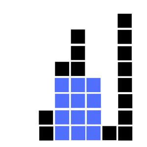
Fence Problem.png

This problem is pretty neat and clean to solve with Haskell, as it lends itself to a recursive solution. First let's define a couple newtypes to illustrate our concepts for this problem. We'll use a compiler extension to derive the Num typeclass on our index type, as this will be useful later.

{-# LANGUAGE GeneralizedNewtypeDeriving #-}
...
newtype FenceValues = FenceValues { unFenceValues :: [Int] }
newtype FenceIndex = FenceIndex { unFenceIndex :: Int }
  deriving (Eq, Num, Ord)
-- Left Index is inclusive, right index is non-inclusive 
newtype FenceInterval = FenceInterval { unFenceInterval :: (FenceIndex, FenceIndex) }
newtype FenceSolution = FenceSolution { unFenceSolution :: Int }
  deriving (Eq, Show, Ord)

Next, we'll define our primary function. It will take our FenceValues, a list of integers, and return our solution.

largestRectangle :: FenceValues -> FenceSolution
largestRectangle values = ...

It in turn will call our recursive helper function. This function will calculate the largest rectangle over a specific interval. We can solve it recursively by using smaller and smaller intervals. We'll start by calling it on the interval of the whole list.

largestRectangle :: FenceValues -> FenceSolution
largestRectangle values = largestRectangleAtIndices values
  (FenceInterval (FenceIndex 0, FenceIndex (length (unFenceValues values))))

largestRectangleAtIndices :: FenceValues -> FenceInterval -> FenceSolution
largestRectangleAtIndices = ...

Now, to break this into recursive cases, we need some more information first. What we need is the index i of the minimum height in this interval. One option is that we could make a rectangle spanning the whole interval with this height.

Any other "largest rectangle" won't use this particular index. So we can then divide our problem into two more cases. In the first, we'll find the largest rectangle on the interval to the left. In the second, we'll look to the right.

As your might realize, these two cases simply involve making recursive calls! Then we can easily compare their results. The only thing we need to add is a base case. Here are all these cases represented in code:

largestRectangleAtIndices :: FenceValues -> FenceInterval -> FenceSolution
largestRectangleAtIndices
  values
  interval@(FenceInterval (leftIndex, rightIndex)) = 
    -- Base Case: Checks if left + 1 >= right
    if isBaseInterval interval
      then FenceSolution (valueAtIndex values leftIndex)
      -- Compare three cases
      else max (max middleCase leftCase) rightCase
      where
      -- Find the minimum height and its index
      (minIndex, minValue) = minimumHeightIndexValue values interval
      -- Case 1: Use the minimum index
      middleCase = FenceSolution $ (intervalSize interval) * minValue
      -- Recursive call #1
      leftCase = largestRectangleAtIndices values (FenceInterval (leftIndex, minIndex))
      -- Guard against case where there is no "right" interval
      rightCase = if minIndex + 1 == rightIndex
        then FenceSolution (minBound :: Int) -- Supply a "fake" solution that we'll ignore
        -- Recursive call #2
        else largestRectangleAtIndices values (FenceInterval (minIndex + 1, rightIndex))

And just like that, we're actually almost finished. The only sticking point here is a few helper functions. Three of these are simple:

valueAtIndex :: FenceValues -> FenceIndex -> Int
valueAtIndex values index = (unFenceValues values) !! (unFenceIndex index)

isBaseInterval :: FenceInterval -> Bool
isBaseInterval (FenceInterval (FenceIndex left, FenceIndex right)) = left + 1 >= right

intervalSize :: FenceInterval -> Int
intervalSize (FenceInterval (FenceIndex left, FenceIndex right)) = right - left

Now we have to determine the minimum on this interval. Let's do this in the most naive way, by scanning the whole interval with a fold.

minimumHeightIndexValue :: FenceValues -> FenceInterval -> (FenceIndex, Int)
minimumHeightIndexValue values (FenceInterval (FenceIndex left, FenceIndex right)) =
  foldl minTuple (FenceIndex (-1), maxBound :: Int) valsInInterval
  where
    valsInInterval :: [(FenceIndex, Int)]
    valsInInterval = drop left (take right (zip (FenceIndex <$> [0..]) (unFenceValues values)))
    minTuple :: (FenceIndex, Int) -> (FenceIndex, Int) -> (FenceIndex, Int)
    minTuple old@(_, heightOld) new@(_, heightNew) =
      if heightNew < heightOld then new else old

And now we're done! As an exercise you can head to this unit test module and write some HUnit tests for this function. Write a few basic tests at first, and then incorporate a test case for the input10000 and output10000 expressions in the file. Run the tests with this command:

>> stack build Testing:test:fences-tests

BENCHMARKING OUR CODE

Now, this is a neat little algorithmic solution, but we want to know if our code is efficient. We need to know if it will scale to larger input values. If you incorporated the size-10000 example into your unit tests, you may have found that the test suite is suddenly quite a bit slower.

We can find the answer to these performance questions by writing benchmarks. Benchmarks are a feature we can use in conjunction with Cabal and Stack. They work a lot like test suites. But instead of proving the correctness of our code, they'll show us how fast our code runs under various circumstances. We'll use the Criterion library to do this. We'll start by adding a section in our .cabal file for this benchmark:

benchmark fences-benchmark
  type:                exitcode-stdio-1.0
  hs-source-dirs:      benchmark
  main-is:             FencesBenchmark.hs
  build-depends:       base
                     , Testing
                     , criterion
                     , random
  default-language:    Haskell2010

Now we'll look at our FencesBenchmark file, make it a Main module and add a main function. We'll start by generating 6 lists, increasing in size by a factor of 10 each time.

module Main where

import Criterion
import Criterion.Main (defaultMain)
import System.Random

import Fences

main :: IO ()
main = do
  [l1, l2, l3, l4, l5, l6] <- mapM 
    randomList [1, 10, 100, 1000, 10000, 100000]
  ...

-- Generate a list of a particular size
randomList :: Int -> IO FenceValues
randomList n = FenceValues <$> (sequence $ replicate n (randomRIO (1, 10000 :: Int)))

Now the syntax for the Criterion library is a lot like HUnit in many respects. It has a defaultMain function. The Benchmark type is a lot like the TestTree type. We can create a single Benchmark using the bench expression, and combine a group of them with bGroup:

main :: IO ()
main = do
  [l1, l2, l3, l4, l5, l6] <- mapM 
    randomList [1, 10, 100, 1000, 10000, 100000]
  defaultMain
    [ bgroup "fences tests" 
      [ bench "Size 1 Test" $ ...
      , bench "Size 10 Test" $ ...
      ]
    ]

The difference is that instead of filling in each case with a test predicate assertion, we can fill it in with a Benchmarkable element. We create these by taking a code expression we want to benchmark (like a call to largestRectangle) and passing it to the whnf function.

main :: IO ()
main = do
  [l1, l2, l3, l4, l5, l6] <- mapM 
    randomList [1, 10, 100, 1000, 10000, 100000]
  defaultMain
    [ bgroup "fences tests" 
      [ bench "Size 1 Test" $ whnf largestRectangle l1
      , bench "Size 10 Test" $ whnf largestRectangle l2
      , bench "Size 100 Test" $ whnf largestRectangle l3
      , bench "Size 1000 Test" $ whnf largestRectangle l4
      , bench "Size 10000 Test" $ whnf largestRectangle l5
      , bench "Size 100000 Test" $ whnf largestRectangle l6
      ]
    ]

That's all there is to it really! We're ready to run our benchmark now. We'd normally run all our benchmarks with stack bench (or cabal bench if you're not using Stack). And you can run an individual benchmark set similar to an individual test set:

>> stack build Testing:bench:fences-benchmark

But we can also compile our code with the --profile flag. This will automatically create a profiling report with more information about our code. Note using profiling requires re-compiling ALL the dependencies to use profiling as well. So you don't want to switch back and forth a lot.

>> stack build Testing:bench:fences-benchmark --profile
Benchmark fences-benchmark: RUNNING...
benchmarking fences tests/Size 1 Test
time                 47.79 ns   (47.48 ns .. 48.10 ns)
                     1.000 R²   (0.999 R² .. 1.000 R²)
mean                 47.78 ns   (47.48 ns .. 48.24 ns)
std dev              1.163 ns   (817.2 ps .. 1.841 ns)
variance introduced by outliers: 37% (moderately inflated)

benchmarking fences tests/Size 10 Test
time                 3.324 μs   (3.297 μs .. 3.356 μs)
                     0.999 R²   (0.999 R² .. 1.000 R²)
mean                 3.340 μs   (3.312 μs .. 3.368 μs)
std dev              98.52 ns   (79.65 ns .. 127.2 ns)
variance introduced by outliers: 38% (moderately inflated)

benchmarking fences tests/Size 100 Test
time                 107.3 μs   (106.3 μs .. 108.2 μs)
                     0.999 R²   (0.999 R² .. 0.999 R²)
mean                 107.2 μs   (106.3 μs .. 108.4 μs)
std dev              3.379 μs   (2.692 μs .. 4.667 μs)
variance introduced by outliers: 30% (moderately inflated)

benchmarking fences tests/Size 1000 Test
time                 8.724 ms   (8.596 ms .. 8.865 ms)
                     0.998 R²   (0.997 R² .. 0.999 R²)
mean                 8.638 ms   (8.560 ms .. 8.723 ms)
std dev              228.8 μs   (193.6 μs .. 272.8 μs)

benchmarking fences tests/Size 10000 Test
time                 909.2 ms   (899.3 ms .. 914.1 ms)
                     1.000 R²   (1.000 R² .. 1.000 R²)
mean                 915.1 ms   (914.6 ms .. 915.8 ms)
std dev              620.1 μs   (136.0 as .. 664.8 μs)
variance introduced by outliers: 19% (moderately inflated)

benchmarking fences tests/Size 100000 Test
time                 103.9 s    (91.11 s .. 117.3 s)
                     0.997 R²   (0.997 R² .. 1.000 R²)
mean                 107.3 s    (103.7 s .. 109.4 s)
std dev              3.258 s    (0.0 s .. 3.702 s)
variance introduced by outliers: 19% (moderately inflated)

Benchmark fences-benchmark: FINISH

So when we run this, we'll find something...troubling. It takes a looong time to run the final benchmark on size 100000. On average, this case takes over 100 seconds...more than a minute and a half! We can further take note of how the average run time increases based on the size of the case. Let's pare down the data a little bit:

Size 1: 47.78 ns
Size 10: 3.340 μs (increased ~70x)
Size 100: 107.2 μs (increased ~32x)
Size 1000: 8.638 ms (increased ~81x)
Size 10000: 915.1 ms (increased ~106x)
Size 100000: 107.3 s (increased ~117x)

Each time we increase the size of the problem by a factor of 10, the time spent increased by a factor closer to 100! This suggests our run time is O(n^2) (check out this guide if you are unfamiliar with Big-O notation). We'd like to do better.

DETERMINING THE PROBLEM

So we want to figure out why our code isn't performing very well. Luckily, we already profiled our benchmark!. This outputs a specific file that we can look at, called fences-benchmark.prof. It has some very interesting results:

COST CENTRE                            MODULE SRC                 %time %alloc
minimumHeightIndexValue.valsInInterval Lib    src/Lib.hs:45:5-95   69.8   99.7
valueAtIndex                           Lib    src/Lib.hs:51:1-74   29.3    0.0

We see that we have two big culprits taking a lot of time. First, there is our function that determines the minimum between a specific interval. The report is even more specific, calling out the specific offending part of the function. We spend a lot of time getting the different values for a specific interval. In second place, we have valueAtIndex. This means we also spend a lot of time getting values out of our list.

First let's be glad we've factored our code well. If we had written our entire solution in one big function, we wouldn't have any leads here. This makes it much easier for us to analyze the problem. When examining the code, we see why both of these functions could produce O(n^2) behavior.

Due to the number of recursive calls we make, we'll call each of these functions O(n) times. Then when we call valueAtIndex, we use the (!!) operator on our linked list. This takes O(n) time. Scanning the whole interval for the minimum height has the same effect. In the worst case, we have to look at every element in the list! I'm hand waving a bit here, but that is the basic result. When we call these O(n) pieces O(n) times, we get O(n^2) time total.

CLIFF HANGER ENDING

We can actually solve this problem in O(n log n) time, a dramatic improvement over the current O(n^2). But we'll have to improve our data structures to accomplish this. First, we'll store our values so that we can go from the index to the element in sub-linear time. This is easy. Second, we have to determine the index containing the minimum element within an arbitrary interval. This is a bit trickier to do in sub-linear time. We'll need a more advanced data structure. To see how this all works, you'll need to check out part 3, the grand finale of this series!

As a reminder, you shold take a look at our mini-course on Stack. It'll teach you the basics of laying out a project and running commands on it using the Stack tool. You should enroll in the Monday Morning Haskell Academy to sign up! Once you know about Stack, it'll be a lot easier to try this problem out for yourself!

In addition to Stack, recursion also featured pretty heavily in our solution here. If you've done any amount of functional programming you've seen recursion in action. But if you want to solidify your knowledge, you should download our Recursion Workbook! It has two chapters worth of content on recursion and it has 10 practice problems you can work through! It also has a full test suite already, so you can use incremental test driven development!

Improving Performance with Data Structures

Welcome to the third and final part of our Haskell testing series! In part 2, we wrote a solution to the "largest rectangle" problem. We implemented benchmarks to determine how well our code performs on certain inputs. First we used the Criterion library to get some measurements for our code. Then we were able to look at those measurements in some spiffy output. We also profiled our code to try to determine what part was slowing us down.

The profiling output highlighted two functions that were taking an awful lot of time. When we analyzed them, we found they were very inefficient. In this article, we'll resolve those problems and improve our code in a couple different ways. First, we'll use an array rather than a list to make our value accesses faster. Then, we'll add a cool data structure called a segment tree. This will help us to quickly get the smallest height value over a particular interval.

The code examples in this article series make good use of the Stack tool. If you've never used Stack before, you should check out our FREE Stack mini-course. It'll walk you through the basics of organizing your code, getting dependencies, and running commands.

Hopefully you've been following the Github Repository for this series! The improved code for this article can be found in the FencesFast module! You can also try re-doing some of these examples for yourself in a Test-Driven-Development style by working in this practice module with these unit tests!

WHAT WENT WRONG?

So first let's take some time to remind ourselves why our solution was inefficient. Both our minimum height function and our "value at index" function ran in O(n) time. This means each of them could scan the entire list in the worst case. Next we observed that both of these functions will get called O(n) times. Thus our total algorithm will be O(n^2) time. The time benchmarks we took backed up this theory. Increasing our input size by a factor of 10 would often result in the solution taking 100 times longer.

The data structures we mentioned in the intro will help us get the values we need without doing a full scan. We'll start with the easier step, substituting an array for our list of values.

ARRAYS

Linked lists are very common when we're solving functional programming problems. They have some nice properties, and work very well with recursion. However, they do not allow fast access by index. For these situations, we need to use arrays. Arrays aren't as common in Haskell as other languages, and there are a few differences.

First, Haskell arrays have two type parameters. When you make an array in Java, you say whether it's an int array (int[]) or a string array (String[]), or whatever other type. So this is only a single parameter. Whenever we want to index into the array, we always use integers.

In Haskell, we get to choose both the type that the array stores AND the type that indexes the array. Now, the indexing type has to belong to the index (Ix) typeclass. And in this case we'll be using Int anyways. But it's cool to know that you have more flexibility. For instance, consider representing a matrix. In Java, we have to use an "array of arrays". This involves a lot of awkward syntax. In Haskell, we can instead use a single array indexed by tuples of integers! Accessing a Matrix with index (2, 1) feels a bit more natural than matrix[2][1]. We could also do something like index from 1 instead of 0 if the situation called for it.

So for our problem, we'll use Array Int Int for our inner fence values instead of a normal list. We'll only need to make a few code changes though! First, we'll import a couple modules and change our type to use the array:

import Data.Array
import Data.Ix (range)

...

newtype FenceValues = FenceValues { unFenceValues :: Array Int Int }

Next, instead of using (!!) to access by index, we'll use the specialized array index (!) operator to access them.

valueAtIndex :: FenceValues -> FenceIndex -> Int
valueAtIndex values index = (unFenceValues values) ! (unFenceIndex index)

Finally, let's improve our minimumHeight function. We'll now use the range function on our array instead of resorting to drop and take. Note we now use right - 1 since we want to exclude the right endpoint of the interval.

where
  valsInInterval :: [(FenceIndex, Int)]
  valsInInterval = zip 
    (FenceIndex <$> intervalRange) 
    (map ((unFenceValues values) !) intervalRange)
    where
      intervalRange = range (left, right - 1)

We'll also have to change our benchmarking code to produce arrays instead of lists. (You can see these updates in the Fast benchmark:

import Data.Array (listArray)

...

randomList :: Int -> IO FenceValues
randomList n = FenceValues . mkListArray <$> 
  (sequence $ replicate n (randomRIO (1, 10000 :: Int)))
  where
    mkListArray vals = listArray (0, (length vals) - 1) vals

Both our library and our benchmark now need to use array in their build-depends section of the Cabal file. We need to make sure we add this! Once we have, we can benchmark our code again, and we'll find it's already sped up quite a bit!

>> stack build Testing:bench:fences-fast-benchmark --profile
Running 1 benchmarks...
Benchmark fences-fast-benchmark: RUNNING...
benchmarking fences tests/Size 1 Test
time                 49.33 ns   (48.98 ns .. 49.71 ns)
                     1.000 R²   (0.999 R² .. 1.000 R²)
mean                 49.46 ns   (49.16 ns .. 49.86 ns)
std dev              1.105 ns   (861.0 ps .. 1.638 ns)
variance introduced by outliers: 33% (moderately inflated)

benchmarking fences tests/Size 10 Test
time                 4.541 μs   (4.484 μs .. 4.594 μs)
                     0.999 R²   (0.998 R² .. 1.000 R²)
mean                 4.496 μs   (4.456 μs .. 4.531 μs)
std dev              132.0 ns   (109.6 ns .. 164.3 ns)
variance introduced by outliers: 36% (moderately inflated)

benchmarking fences tests/Size 100 Test
time                 79.81 μs   (79.21 μs .. 80.45 μs)
                     0.999 R²   (0.999 R² .. 1.000 R²)
mean                 79.51 μs   (78.93 μs .. 80.39 μs)
std dev              2.396 μs   (1.853 μs .. 3.449 μs)
variance introduced by outliers: 29% (moderately inflated)

benchmarking fences tests/Size 1000 Test
time                 1.187 ms   (1.158 ms .. 1.224 ms)
                     0.995 R²   (0.992 R² .. 0.998 R²)
mean                 1.170 ms   (1.155 ms .. 1.191 ms)
std dev              56.61 μs   (48.02 μs .. 70.28 μs)
variance introduced by outliers: 37% (moderately inflated)

benchmarking fences tests/Size 10000 Test
time                 15.03 ms   (14.71 ms .. 15.32 ms)
                     0.997 R²   (0.994 R² .. 0.999 R²)
mean                 15.71 ms   (15.44 ms .. 16.03 ms)
std dev              729.7 μs   (569.3 μs .. 965.4 μs)
variance introduced by outliers: 16% (moderately inflated)

benchmarking fences tests/Size 100000 Test
time                 191.4 ms   (189.2 ms .. 193.9 ms)
                     1.000 R²   (1.000 R² .. 1.000 R²)
mean                 189.3 ms   (188.2 ms .. 190.5 ms)
std dev              1.471 ms   (828.0 μs .. 1.931 ms)
variance introduced by outliers: 14% (moderately inflated)

Benchmark fences-fast-benchmark: FINISH

Here's what the multiplicative factors are:

Size 1: 49.33 ns
Size 10: 4.451 μs (increased ~90x)
Size 100: 79.81 μs (increased ~18x)
Size 1000: 1.187 ms (increased ~15x)
Size 10000: 15.03 ms (increased ~13x)
Size 100000: 191.4 ms (increased ~13x)

For the later cases, increasing size by a factor 10 seems to only increase the time by a factor of 13-15. We could be forgiven for thinking we have achieved O(n log n) time already!

DIFFERENT TEST CASES

But something still doesn't sit right. We have to remember that the theory doesn't quite justify our excitement here. In fact our old code was so bad that the NORMAL case was O(n^2). Now it seems like we may have gotten O(n log n) for the average case. But we want to prepare for the worst case if we can. In this situation, our code will not be so performant when the lists of input heights is sorted!

main :: IO ()
main = do
  [l1, l2, l3, l4, l5, l6] <- mapM 
    randomList [1, 10, 100, 1000, 10000, 100000]
  let l7 = sortedList
  defaultMain
    [ bgroup "fences tests" 
       ...
      , bench "Size 100000 Test" $ whnf largestRectangle l6
      , bench "Size 100000 Test (sorted)" $ whnf largestRectangle l7
      ]
    ]

...

sortedList :: FenceValues
sortedList = FenceValues $ listArray (0, 99999) [1..100000]

We'll once again find that this last case takes a loooong time, and we'll see a big spike in run time.

>> stack build Testing:bench:fences-fast-benchmark --profile
Running 1 benchmarks...
Benchmark fences-fast-benchmark: RUNNING...

...

benchmarking fences tests/Size 100000 Test (sorted)
time                 378.1 s    (355.0 s .. 388.3 s)
                     1.000 R²   (0.999 R² .. 1.000 R²)
mean                 384.5 s    (379.3 s .. 387.2 s)
std dev              4.532 s    (0.0 s .. 4.670 s)
variance introduced by outliers: 19% (moderately inflated)

Benchmark fences-fast-benchmark: FINISH

It averages more than 6 minutes per case! But this time, we'll see the profiling output has changed. It only calls out various portions of minimumHeightIndexValue! We no longer spend a lot of time in valueAtIndex.

COST CENTRE                                          %time %alloc

minimumHeightIndexValue.valsInInterval               65.0   67.7
minimumHeightIndexValue                              22.4    0.0
minimumHeightIndexValue.valsInInterval.intervalRange 12.4   32.2

So now we have to solve this new problem by improving our calculation of the minimum.

SEGMENT TREES

Our current approach still requires us to look at every element in our interval. Even though some of our intervals will be small, there will be a lot of these smaller calls, so the total time is still O(n^2). We need a way to find the smallest item and value on a given interval without resorting to a linear scan.

One idea would be to develop an exhaustive list of all the answers to this question right at the start. We could make a mapping from all possible intervals to the smallest index and value in the interval. But this won't help us in the end. There are still n^2 possible intervals. So creating this data structure will still mean that our code takes O(n^2) time.

But we're on the right track with the idea of doing some of the work before hand. We'll have to use a data structure that's not an exhaustive listing though. Enter segment trees.

A segment tree has the same structure as a binary search tree. Instead of storing a single value though, each node corresponds to an interval. Each node will store its interval, the smallest value over that interval, and the index of that value.

The top node on the tree will refer to the interval of the whole array. It'll store the pair for the smallest value and index overall. Then it will have two children nodes. The left one will have the minimum pair over the first half of the tree, and the right one will have the second half. The next layer will break it up into quarters, and so on.

As an example, let's consider how we would determine the minimum pair starting from the first quarter point and ending at the third quarter point. We'll do this using recursion. First, we'll ask the left subtree for the minimum pair on the interval from the quarter point to the half point. Then we'll query the right tree for the smallest pair from the half point to the three-quarters point. Then we can take the smallest of those and return it. I won't go into all the theory here, but it turns out that even in the worst case this operation takes O(log n) time.

DESIGNING OUR SEGMENT TREE

There is a library called Data.SegmentTree on hackage. But our code is short and specialized enough that we can do this from scratch. We'll compose our tree from SegmentTreeNodes. Each node is either empty, or it contains six fields. The first two refer to the interval the node spans. The next will be the minimum value and the index of that value over the interval. And then we'll have fields for each of the children nodes of this node:

data SegmentTreeNode = ValueNode
  { fromIndex :: FenceIndex
  , toIndex :: FenceIndex
  , value :: Int
  , minIndex :: FenceIndex
  , leftChild :: SegmentTreeNode
  , rightChild :: SegmentTreeNode
  }
  | EmptyNode

We could make this Segment Tree type a lot more generic so that it isn't restricted to our fence problem. I would encourage you to take this code and try that as an exercise!

BUILDING THE SEGMENT TREE

Now we'll add our preprocessing step where we'll actually build the tree itself. This will use the same interval/tail pattern we saw before. In the base case, the interval's span is only 1, so we make a node containing that value with empty sub-children. We'll also add a catchall that returns an EmptyNode:

buildSegmentTree :: Array Int Int -> SegmentTreeNode
buildSegmentTree ints = buildSegmentTreeTail 
  ints 
  (FenceInterval ((FenceIndex 0), (FenceIndex (length (elems ints)))))

buildSegmentTreeTail :: Array Int Int -> FenceInterval -> SegmentTreeNode
buildSegmentTreeTail array
  (FenceInterval (wrappedFromIndex@(FenceIndex fromIndex), wrappedToIndex@(FenceIndex toIndex)))
  | fromIndex + 1 == toIndex = ValueNode 
      { fromIndex = wrappedFromIndex
      , toIndex = wrappedToIndex
      , value = array ! fromIndex
      , minIndex = wrappedFromIndex
      , leftChild = EmptyNode
      , rightChild = EmptyNode
      }
  | ... TODO
  | otherwise = EmptyNode

Now our middle case will be the standard case. First we'll divide our interval in half and make two recursive calls.

where 
  average = (fromIndex + toIndex) `quot` 2
  -- Recursive Calls
  leftChild = buildSegmentTreeTail 
    array (FenceInterval (wrappedFromIndex, (FenceIndex average)))
  rightChild = buildSegmentTreeTail 
    array (FenceInterval ((FenceIndex average), wrappedToIndex))

Next we'll write a function that'll extract the minimum value and index, but handle the empty node case. This provided maxBound as the "minimum" so comparisons will always favor the non-empty nodes:

-- Get minimum val and index, but account for empty case.
valFromNode :: SegmentTreeNode -> (Int, FenceIndex)
valFromNode EmptyNode = (maxBound :: Int, FenceIndex (-1))
valFromNode n@ValueNode{} = (value n, minIndex n)

Now, back in buildSegmentTreeTail, we'll compare the three cases for the minimum. It'll likely be the values from the left or the right. Otherwise it's the current value.

where
  ...
  leftCase = valFromNode leftChild
  rightCase = valFromNode rightChild
  currentCase = (array ! fromIndex, wrappedFromIndex)
  (newValue, newIndex) = min (min leftCase rightCase) currentCase

Finally we'll complete our definition by filling in the missing variables in the middle/normal case. You can look at the complete definition here:

buildSegmentTreeTail :: Array Int Int -> FenceInterval -> SegmentTreeNode
buildSegmentTreeTail array
  (FenceInterval (wrappedFromIndex@(FenceIndex fromIndex), wrappedToIndex@(FenceIndex toIndex)))
  | ... -- base case
  | fromIndex < toIndex = ValueNode 
    { fromIndex = wrappedFromIndex
    , toIndex = wrappedToIndex
    , value = newValue
    , minIndex = newIndex
    , leftChild = leftChild
    , rightChild = rightChild
    }
  | otherwise = EmptyNode
    where 
      average = ...
      leftChild = ...
      rightChild = ...

      leftCase = valFromNode leftChild
      rightCase = valFromNode rightChild
      currentCase = (array ! fromIndex, wrappedFromIndex)
      (newValue, newIndex) = min (min leftCase rightCase) currentCase

valFromNode :: SegmentTreeNode -> (Int, FenceIndex)
valFromNode = ...

FINDING THE MINIMUM

Now let's write the critical function of finding the minimum over the given interval. This will be like our slower version, but we'll add our tree as another parameter. Then we'll handle the EmptyNode case in the same way as above. Then we can unwrap our values for the full case:

minimumHeightIndexValue :: FenceValues -> SegmentTreeNode -> FenceInterval -> (FenceIndex, Int)
minimumHeightIndexValue values tree 
  originalInterval@(FenceInterval (FenceIndex left, FenceIndex right)) =
  case tree of
    EmptyNode -> (maxBound :: Int, -1)
    ValueNode
      { fromIndex = FenceIndex nFromIndex
      , toIndex = FenceIndex nToIndex
      , value = nValue
      , minIndex = nMinIndex
      , leftChild = nLeftChild
      , rightChild = nRightChild} -> ...

The first case we'll handle is that the current node exactly matches the interval we are passed. Obviously we can simply supply the value and index here:

case tree of
  ValueNode
    { fromIndex = FenceIndex nFromIndex
    , toIndex = FenceIndex nToIndex
    , value = nValue
    , minIndex = nMinIndex
    , ... } -> if left == nFromIndex && right == nToIndex 
      then (nMinIndex, nValue)
      else ...

Next we'll observe two cases that will need only one recursive call. If the right index is below the midway point, we recursively call to the left sub-child. And if the left index is above the midway point, we'll call on the right side (we'll calculate the average later).

case tree of
  ValueNode
    { ... } -> if left == nFromIndex && right == nToIndex 
      then (nMinIndex, nValue)
      else if right < average 
        then minimumHeightIndexValue values nLeftChild originalInterval
        else if left >= average
          then minimumHeightIndexValue values nRightChild originalInterval
          else ...
        where
          average = (nFromIndex + nToIndex) `quot` 2

Finally we have the tricky part. If the interval does cross the halfway mark, we'll have to divide it into two sub-intervals. Then we'll make two recursive calls, and get their solutions. Finally, we'll compare the two solutions and take the smaller one. This requires the definition of one more helper function minTuple, to compare indices by their corresponding heights.

case tree of
  ValueNode
    { ... } -> if left == nFromIndex && right == nToIndex 
      then (nMinIndex, nValue)
      else if right < average 
        then ... -- left recursive case
        else if left >= average
          then ... -- right recursive case
          else minTuple leftResult rightResult
        where
          average = (nFromIndex + nToIndex) `quot` 2
          leftResult = minimumHeightIndexValue values nLeftChild
            (FenceInterval (FenceIndex left, FenceIndex average))
          rightResult = minimumHeightIndexValue values nRightChild
            (FenceInterval (FenceIndex average, FenceIndex right))
          minTuple :: (FenceIndex, Int) -> (FenceIndex, Int) -> (FenceIndex, Int)
          minTuple old@(_, heightOld) new@(_, heightNew) =
            if heightNew < heightOld then new else old

Again, you can see the complete function here.

TOUCHING UP THE REST

Once we've accomplished this, the rest is pretty straightforward. First, we'll build our segment tree at the beginning and pass it as a parameter to our function. Then we'll plug in our new minimum function in place of the old one. We'll make sure to add the tree to each recursive call as well.

largestRectangle :: FenceValues -> FenceSolution
largestRectangle values = largestRectangleAtIndices values 
  (buildSegmentTree (unFenceValues values))
  (FenceInterval (FenceIndex 0, FenceIndex (length (unFenceValues values))))

...
-- Notice the extra parameter
largestRectangleAtIndices :: FenceValues -> SegmentTreeNode -> FenceInterval -> FenceSolution
largestRectangleAtIndices
  values
  tree
...
      where
      ...
      -- And down here add it to each call
      (minIndex, minValue) = minimumHeightIndexValue values tree interval
      leftCase = largestRectangleAtIndices values tree (FenceInterval (leftIndex, minIndex))
      rightCase = if minIndex + 1 == rightIndex
        then FenceSolution (maxBound :: Int)
        else largestRectangleAtIndices values tree (FenceInterval (minIndex + 1, rightIndex))

And now we can run our benchmark again. This time, we'll see that our code runs a great deal faster on both large cases! Success!

benchmarking fences tests/Size 100000 Test
time                 179.1 ms   (173.5 ms .. 185.9 ms)
                     0.999 R²   (0.998 R² .. 1.000 R²)
mean                 184.1 ms   (182.7 ms .. 186.1 ms)
std dev              2.218 ms   (1.197 ms .. 3.342 ms)
variance introduced by outliers: 14% (moderately inflated)

benchmarking fences tests/Size 100000 Test (sorted)
time                 238.4 ms   (227.2 ms .. 265.1 ms)
                     0.998 R²   (0.989 R² .. 1.000 R²)
mean                 243.5 ms   (237.0 ms .. 251.8 ms)
std dev              8.691 ms   (2.681 ms .. 11.83 ms)
variance introduced by outliers: 16% (moderately inflated)

CONCLUSION

So in this series, we learned a whole lot. In part 1, we talked about the basic ideas behind test driven development and some Haskell unit testing libraries. In part 2, we then covered how to create benchmarks for our code using Cabal/Stack. When we ran those benchmarks, we found results took longer than we would like. We then used profiling to determine what the problematic functions were.

To solve the problems we found, we dove head-first into some data structures knowledge. We saw first hand how changing the underlying data structures of our program could improve our performance. We also learned about arrays, which are somewhat overlooked in Haskell. Then we built a segment tree from scratch and used its API to enable our program's improvements.

If you want some extra practice with Test Driven Development, benchmarks, and our Fence example, you can take a look at our practice module and corresponding practice test suite. You can solve the most important parts of the algorithm using TDD and writing your test cases as you go along!

This problem involved many different uses of recursion. If you want to become a better functional programmer, you'd better learn recursion. If you want a better grasp of this fundamental concept, you should check out our free Recursion Workbook. It has two chapters of useful information as well as 10 practice problems!

Finally, be sure to check out our Stack mini-course. Once you've mastered the Stack tool, you'll be well on your way to making Haskell projects like a Pro!

Haskell's Data Types!

PART 1: HASKELL'S SIMPLE DATA TYPES

I first learned about Haskell in college. I've considered why I kept up with Haskell after, even when I didn't know about its uses in industry. I realized there were a few key elements that drew me to it.

In a word, Haskell is elegant. For me, this means we can simple concepts in simple terms. In this series, we're going to look at some of these concepts. We'll see that Haskell expresses a lot of ideas in simple terms that other languages express in more complicated terms. In the first part, we'll start by looking at simple data declarations. If you're already familiar with Haskell data declarations, you can move onto part 2, where we'll talk about sum types!

If you've never used Haskell, now is the perfect time to start! For a quick start guide, download our Beginners Checklist. For a more in-depth walkthrough, read our Liftoff Series!

Like some of our other beginner-level series, this series has a companion Github Repository. All the code in these articles lives there so you can follow along and try out some changes if you want! For this article you can look at the Haskell definitions here, or the Java code, or the Python example.

HASKELL DATA DECLARATIONS

To start this series, we'll be comparing a data type with a single constructor across a few different languages. In the next part, we'll look at multi-constructor types. So let's examine a simple type declaration:

data SimplePerson = SimplePerson String String String Int String

Our declaration is very simple, and fits on one line. There's a single constructor with a few different fields attached to it. We know exactly what the types of those fields are, so we can build the object. The only way we can declare a SimplePerson is to provide all the right information in order.

firstPerson :: SimplePerson
firstPerson = SimplePerson "Michael" "Smith" "msmith@gmail.com" 32 "Lawyer"

If we provide any less information, we won't have a SimplePerson! We can leave off the last argument. But then the resulting type reflects that we still need that field to complete our item:

incomplete :: String -> SimplePerson
incomplete = SimplePerson "Michael" "Smith" "msmith@gmail.com" 32

complete :: SimplePerson
complete = incomplete "Firefighter"

Now, our type declaration is admittedly confusing. We don't know what each field means at all when looking at it. And it would be easy to mix things up. But we can fix that in Haskell with record syntax, which assigns a name to each field.

data Person = Person
  { personFirstName :: String
  , personLastName :: String
  , personEmail :: String
  , personAge :: Int
  , personOccupation :: String
  }

We can use these names as functions to retrieve the specific fields out of the data item later.

fullName :: Person -> String
fullName person = personFirstName person ++ " "
  ++ personLastName person

With either construction though, we can also use a pattern match to retrieve the relevant information.

fullNameSimple :: SimplePerson -> String
fullNameSimple (SimplePerson fn ln _ _ _) = fn ++ " " ++ ln

fullName' :: Person -> String
fullName' (Person fn ln _ _ _) = fn ++ " " ++ ln

And that's the basics of data types in Haskell! Let's take a look at this same type declaration in a couple other languages.

JAVA

If we wanted to express this in the simplest possible Java form, we'd do so like this:

public class Person {
  public String firstName;
  public String lastName;
  public String email;
  public int age;
  public String occupation;
}

Now, this definition isn't much longer than the Haskell definition. It isn't a very useful definition as written though! We can only initialize it with a default constructor Person(). And then we have to assign all the fields ourselves! So let's fix this with a constructor:

public class Person {
    public String firstName;
    public String lastName;
    public String email;
    public int age;
    public String occupation;

    public Person(String fn,
                  String ln, 
                  String em, 
                  int age, 
                  String occ) {
        this.firstName = fn;
        this.lastName = ln;
        this.email = em;
        this.age = age;
        this.occupation = occ;
    }
}

Now we can initialize it in a sensible way. But this still isn't idiomatic Java. Normally, we would have our instance variables declared as private, not public. Then we would expose the ones we wanted via "getter" and "setter" methods. If we do this for all our types, it would bloat the class quite a bit. In general though, you wouldn't have arbitrary setters for all your fields. Here's our code with getters and one setter.

public class Person {
    private String firstName;
    private String lastName;
    private String email;
    private int age;
    private String occupation;

    public Person(String fn, 
                  String ln, 
                  String em,
                  int age,
                  String occ) {
        this.firstName = fn;
        this.lastName = ln;
        this.email = em;
        this.age = age;
        this.occupation = occ;
    }

  public String getFirstName() { return this.firstName; }
  public String getLastName() { return this.lastName; }
  public String getEmail() { return this.email; }
  public int getAge() { return this.age; }
  public String getOccupation() { return this.occupation; }

  public void setOccupation(String occ) { this.occupation = occ; }
}

Now we've got code that is both complete and idiomatic Java.

PUBLIC AND PRIVATE

We can see that the lack of a public/private distinction in Haskell saves us a lot of grief in defining our types. Why don't we do this?

In general, we'll declare our data types so that constructors and fields are all visible. After all, data objects should contain data. And this data is usually only useful if we expose it to the outside world. But remember, it's only exposed as read-only, because our objects are immutable! We'd have to construct another object if we want to "mutate" an existing item (IO monad aside).

The other thing to note is we don't consider functions as a part of our data type in the same way Java (or C++) does. A function is a function whether we define it along with our type or not. So we separate them syntactically from our type, which also contributes to conciseness.

Of course, we do have some notion of public and private items in Haskell. Instead of using the type defintion, we handle it with our module definitins. For instance, we might abstract constructors behind other functions. This allows extra features like validation checks. Here's how we can define our person type but hide it's true constructor:

module Person (Person, mkPerson) where

-- We do NOT export the `Person` constructor!
--
-- To do that, we would use:
-- module Person (Person(Person)) where
--   OR
-- module Person (Person(..)) where

data Person = Person String String String Int String

mkPerson :: String -> String -> String -> Int -> String
  -> Either String Person
mkPerson = ...

Now anyone who uses our code has to use the mkPerson function. This lets us return an error if something is wrong!

PYTHON

As our last example in this article, here's a simple Python version of our data type.

class Person(object):

  def __init__(self, fn, ln, em, age, occ):
    self.firstName = fn
    self.lastName = ln
    self.email = em
    self.age = age
    self.occupation = occ

This definition is pretty compact. We can add functions to this class, or define them outside and pass the class as another variable. It's not as clean as Haskell, but much shorter than Java.

Now, Python has no notion of private member variables. Conventions exist, like using an underscore in front of "private" variable names. But you can't restrict their usage outside of your file, even through imports! This helps keep the type definition smaller. But it does make Python a little less flexible than other languages.

What Python does have is more flexibility in argument ordering. We can name our arugments as follows, allowing us to change the order we use to initialize our type. Then we can include default arguments (like None).

class Person(object):

  def __init__(self, fn=None, ln=None, em=None, age=None, occ=None):
    self.firstName = fn
    self.lastName = ln
    self.email = em
    self.age = age
    self.occupation = occ

# This person won't have a first name!
myPerson = Person(
             ln="Smith",
             age=25,
             em="msmith@gmail.com",
             occ="Lawyer")

This gives more flexibility. We can initialize our object in a lot more different ways. But it's also a bit dangerous. Now we don't necessarily know what fields are null when using our object. This can cause a lot of problems later. We'll explore this theme throughout this series when looking at Python data types and code.

JAVASCRIPT

We'll be making more references to Python throughout this series as we explore its syntax. Most of the observations we make about Python apply equally well to Javascript. In general, Javascript offers us flexibility in constructing objects. For instance, we can even extend objects with new fields once they're created. Javascript even naturalizes the concept of extending objects with functions. (This is possible in Python, but not as idiomatic).

A result of this though is that we have no guarantees about how which of our objects have which fields. We won't know for sure we'll get a good value from calling any given property. Even basic computations in Javascript can give results like NaN or undefined. In Haskell you can end up with undefined, but pretty much only if you assign that value yourself! And in Haskell, we're likely to see an immediate termination of the program if that happens. Javascript might percolate these bad values far up the stack. These can lead to strange computations elsewhere that don't crash our program but give weird output instead!

But the specifics of Javascript can change a lot with the framework you happen to be using. So we won't cite too many code examples in this series. Remember though, most of the observations we make with Python will apply.

CONCLUSION

So after comparing these methods, I much prefer using Haskell's way of defining data. It's clean and quick. We can associate functions with our type or not, and we can make fields private if we want. And that's just in the one-constructor case! We'll see how things get even more hairy for other languages when we add more constructors! Take a look at part 2 to see how things stack up!

If you've never programmed in Haskell, hopefully this series shows you why it's actually not too hard! Read our Liftoff Series or download our Beginners Checklist to get started!

Sum Types in Haskell

Welcome to the second part of our series on Haskell's data types. This is part of an exploration of concepts that are simple to express in Haskell but harder in other languages. In part 1 we began by looking at simple data declarations. In this part, we'll go one step further and look at sum types. That is, we'll consider types with more than one constructor. These allow the same type to represent different kinds of data. They're invaluable in capturing many concepts. In you already know about sum types, you should move onto part 3, where we'll get into parameterized types.

Most of the material in this article is pretty basic. But if you haven't gotten the chance to use Haskell yet, you might to start from the beginning! Download our Beginners Checklist or read our Liftoff Series!

Don't forget you can a look at the code for these articles on our Github Repository! You can look along for reference and try to make some changes as well. For this article you can look at the Haskell code here, or the Java examples), or the Python example.

HASKELL BASIC SUM TYPES

In part 1, we started with a basic Person type like so:

data Person = Person String String String Int String We can expand this type by adding more constructors to it. Let's imagine our first constructor refers to an adult person. Then we could make a second constructor for a Child. It will have different information attached. For instance, we only care about their first name, age, and what grade they're in:

data Person =
  Adult String String String Int String |
  Child String Int Int

To determine what kind of Person we're dealing with, it's a simple case of pattern matching. So whenever we need to branch, we do this pattern match in a function definition or a case statement!

personAge :: Person -> Int
personAge (Adult _ _ _ a _) = a
personAge (Child _ a _) = a

-- OR

personAge :: Person -> Int
personAge p = case p of
  Adult _ _ _ a _ -> a
  Child _ a _ -> a

On the whole, our definition is very simple! And the approach scales. Adding a third or fourth constructor is just as simple! This extensibility is super attractive when designing types. The ease of this concept was a key point in convincing me about Haskell.

RECORD SYNTAX

Before we move onto other languages, it's worth noting the imperfections with this design. In our type above, it can be a bit confusing what each field represents. We used record syntax in the previous part to ease this pain. We can apply that again on this sum type:

data Person2 =
  Adult2
    { adultFirstName :: String
    , adultLastName :: String
    , adultEmail :: String
    , adultAge :: Int
    , adultOccupation :: String
    } |
  Child2
    { childFirstName :: String
    , childAge :: Int
    , childGrade :: Int
    }

This works all right, but it still leaves us with some code smells we don't want in Haskell. In particular, record syntax derives functions for us. Here are a few type signatures of those functions:

adultEmail :: Person -> String
childAge :: Person -> Int
childGrade :: Person -> Int

Unfortunately, these are partial functions. They are only defined for Person2 elements of the proper constructor. If we call adultEmail on a Child, we'll get an error, and we don't like that. The types appear to match up, but it will crash our program! We can work around this a little by merging field names like adultAge and childAge. But at the end of the day we'll still have some differences in what data we need.

-- These compile, but will fail at runtime!
adult2Error :: String
adult2Error = childFirstName adult2

child2Error :: String
child2Error = adultLastName child2

Coding practices can reduce the burden somewhat. For example, it is quite safe to call head on a list if you've already pattern matched that it is non-empty. Likewise, we can use record syntax functions if we're in a "post-pattern-match" situation. But we would need to ignore them otherwise! And this is a rule we would like to avoid in Haskell.

JAVA APPROACH I: MULTIPLE CONSTRUCTORS

Now let's try to replicate the idea of sum types in other languages. It's a little tricky. Here's a first approach we can do in Java. We could set a flag on our type indicating whether it's a Parent or a Child. Then we'll have all the different fields within our type. Note we'll use public fields without getters and setters for the sake of simplicity. Like Haskell, Java allows us to use two different constructors for our type:

public class MultiPerson {
  public boolean isAdult;
  public String adultFirstName;
  public String adultLastName;
  public String adultEmail;
  public int adultAge;
  public String adultOccupation;
  public String childFirstName;
  public int childAge;
  public int childGrade;

  // Adult Constructor
  public MultiPerson(String fn, String ln, String em, int age, String occ) {
    this.isAdult = true;
    this.adultFirstName = fn;
    ...
  }

  // Child Constructor
  public MultiPerson(String fn, int age, int grade) {
    this.isAdult = false;
    this.childFirstName = fn;
    ...
  }
}

We can see that there's a big amount of bloat on the field values, even if we were to combine common ones like age. Then we'll have more awkwardness when writing functions that have to pattern match. Each function within the type will involve a check on the boolean flag. And these checks might also percolate to outer calls as well.

public class MultiPerson {
  ...
  public String getFullName() {
    if (this.isAdult) {
      // Adult Code
    } else {
      // Child Code
    }
  }
}

This approach is harder to scale to more constructors. We would need an enumerated type rather than a boolean for the "flag" value. And it would add more conditions to each of our functions. This approach is cumbersome. It's also very unidiomatic Java code. The more "proper" way involves using inheritance.

JAVA APPROACH II: INHERITANCE

Inheritance is a way of sharing code between types in an object oriented language. For this example, we would make Person a "superclass" of separate Adult and Child classes. We would have separate class declarations for each of them. The Person class would share all the common information. Then the child classes would have code specific to them.

public class Person {
  public String firstName;
  public int age;

  public Person(String fn, int age) {
    this.firstName = fn;
    this.age = age;
  }

  public String getFullName() {
    return this.firstName;
  }
}

// NOTICE: extends Person
public class Adult extends Person {
  public String lastName;
  public String email;
  public String occupation;

  public Adult(String fn, String ln, String em, int age, String occ) {
    // super calls the "Person" constructor
    super(fn, age);
    this.lastName = ln;
    this.email = em;
    this.occupation = occ;
  }

  // Overrides Person definition!
  public String getFullName() {
    return this.firstName + " " + this.lastName;
  }
}

// NOTICE: extends Person
public class Child extends Person {
  public int grade;

  public Child(String fn, int age, int grade) {
    // super calls the "Person" constructor
    super(fn, age);
    this.grade = grade;
  }

  // Does not override getFullName!
}

By extending the Person type, each of our subclasses gets access to the firstName and age fields. We also get access to the getFullName function if we want. However, the Adult subclass chooses to override it.

There's a big upside we get here that Haskell doesn't usually have. In this case, we've encoded the constructor we used with the type. We'll be passing around Adult and Child objects for the most part. This saves a lot of the partial function problems we encounter in Haskell.

We will, on occasion, combine these in a form where we need to do pattern matching. For example, we can make an array of Person objects.

Adult adult = new Adult("Michael", "Smith", "msmith@gmail.com", 32, "Lawyer"); Child child = new Child("Kelly", 8, 2); Person[] people = {adult, child}; Then at some point we'll need to determine which have type Adult and which have type Child. This is possible by using the isinstance condition in Java. But again, it's unidiomatic and we should strive to avoid it. Still, inheritance represents a big improvement over our first approach. Luckily, though, we could still use the getFullName function, and it would work properly for both of them with overriding!

PYTHON: ONLY ONE CONSTRUCTOR!

Unlike Java, Python only allows a single constructor for each type. The way we would control what "type" we make is by passing a certain set of arguments. We then provide None default values for the rest. Here's what it might look like.

class Person(object):
  def __init__(self,
               fn = None,
               ln = None,
               em = None,
               age = None,
               occ = None,
               grade = None):
    if fn and ln and em and age and occ:
      self.isAdult = true
      self.firstName = fn
      self.lastName = ln
      self.age = age
      self.occupation = occ
      self.grade = None
    elif fn and age and grade:
      self.isAdult = false
      self.firstName = fn
      self.age = age
      self.grade = grade
      self.lastName = None
      self.email = None
      self.occupation = None
    else:
      raise ValueError("Failed to construct a Person!")

# Note which arguments we use!
adult = Person(fn="Michael", ln="Smith", em="msmith@gmail.com", age=25, occ="Lawyer")
child = Person(fn="Mike", age=12, grade=7)

But there's a lot of messiness here! A lot of input combinations lead to errors! Because of this, the inheritance approach we proposed for Java is also the best way to go for Python.

class Person():
  def __init__(self, fn, age):
    self.firstName = fn
    self.age = age

  def getFullName(self):
    return self.firstName

class Adult(Person):
  def __init__(self, fn, ln, em, age, occ):
    super().__init__(fn, age)
    self.lastName = ln
    self.email = em
    self.occupation = occ

  def getFullName(self):
    return self.firstName + " " + self.lastName

class Child(Person):
  def __init__(self, fn, age, grade):
    super().__init__(fn, age)
    self.grade = grade

Again though, Python lacks pattern matching across different types of classes. This means we'll have more if statements like if isinstance(x, Adult). In fact, these will be even more prevalent in Python, as type information isn't attached.

COMPARISONS

Once again, we see certain themes arising. Haskell has a clean, simple syntax for this concept. It isn't without its difficulties, but it gets the job done if we're careful. Java gives us a couple ways to manage the issue of sum types. One is cumbersome and unidiomatic. The other is more idiomatic, but presents other issues as we'll see later. Then Python gives us a great deal of flexibility but few guarantees about anything's type. The result is that we can get a lot of errors.

CONCLUSION

In this second part of the series,, we continued our look at the simplicity of constructing types in Haskell. We saw how a first try at replicating the concept of sum types in other languages leads to awkward code. In a couple weeks, we'll dig deeper into the concept of inheritance. It offers a decent way to accomplish our task in Java and Python. And yet, there's a reason we don't have it in Haskell. But first up, the next part will look at the idea of parametric types. We'll see again that it is simpler to do this in Haskell's syntax than other languages. We'll need those ideas to help us explore inheritance later.

If this series makes you want to try Haskell more, it's time to get going! Download our Beginner's Checklist for some tips and tools on starting out! Or read our Liftoff Series for a more in depth look at Haskell basics.

Parameterized Types in Haskell

Welcome back to our series on the simplicity of Haskell's data declarations. In part 2, we looked at how to express sum types in different languages. We saw that they fit very well within Haskell's data declaration system. For Java and Python, we ended up using inheritance, which presents some interesting benefits and drawbacks. We'll explore those more in part 4. But first, we should wrap our heads around one more concept: parametric types.

We'll see how each of these languages allows for the concept of parametric types. In my view, Haskell does have the cleanest syntax. But other compiled languages do pretty well to incorporate the concept. Dynamic languages though, provide insufficient guarantees for my liking.

This all might seem a little wild if you haven't done any Haskell at all yet! Read our Liftoff Series to get started!

As always, you can look at the code for these articles on our Github Repository! For this article you can look at the Haskell example, or the Java code, or the Python example.

HASKELL PARAMETRIC TYPES Let's remember how easy it is to do parametric types in Haskell. When we want to parameterize a type, we'll add a type variable after its name in the definition. Then we can use this variable as we would any other type. Remember our Person type from the first part? Here's what it looks like if we parameterize the occupation field.

data Person o = Person
  { personFirstName :: String
  , personLastName :: String
  , personEmail :: String
  , personAge :: Int
  , personOccupation :: o
  }

We add the o at the start, and then we can use o in place of our former String type. Now whenever we use the Person type, we have to specify a type parameter to complete the definition.

data Occupation = Lawyer | Doctor | Engineer

person1 :: Person String
person1 = Person "Michael" "Smith" "msmith@gmail.com" 27 "Lawyer"

person2 :: Person Occupation
person2 = Person "Katie" "Johnson" "kjohnson@gmail.com" 26 Doctor

When we define functions, we can use a specific version of our parameterized type if we want to constrain it. We can also use a generic type if it doesn't matter.

salesMessage :: Person Occupation -> String
salesMessage p = case personOccupation p of
  Lawyer -> "We'll get you the settlement you deserve"
  Doctor -> "We'll get you the care you need"
  Engineer -> "We'll build that app for you"

fullName :: Person o -> String
fullName p = personFirstName p ++ " " ++ personLastName p

Last of all, we can use a typeclass constraint on the parametric type if we only need certain behaviors:

sortOnOcc :: (Ord o) => [Person o] -> [Person o]
sortOnOcc = sortBy (\p1 p2 -> compare (personOccupation p1) (personOccupation p2))

JAVA GENERIC TYPES

Java has a comparable concept called generics. The syntax for defining generic types is pretty clean. We define a type variable in brackets. Then we can use that variable as a type freely throughout the class definition.

public class Person<T> {
    private String firstName;
    private String lastName;
    private String email;
    private int age;
    private T occupation;

    public Person(String fn, String ln, String em, int age, T occ) {
        this.firstName = fn;
        this.lastName = ln;
        this.email = em;
        this.age = age;
        this.occupation = occ;
    }

    public T getOccupation() { return this.occupation; }
    public void setOccupation(T occ) { this.occupation = occ; }
    ...
}

enum Occupation {
  LAWYER,
  DOCTOR,
  ENGINEER
}

public static void main(String[] args) {
  Person<String> person1 = new Person<String>("Michael", "Smith", "msmith@gmail.com", 27, "Lawyer");
  Person<Occupation> person2 = new Person<Occupation>("Katie", "Johnson", "kjohnson@gmail.com", 26, Occupation.DOCTOR);
}

There's a bit of a wart in how we pass constraints. This comes from the Java distinction of interfaces from classes. Normally, when you define a class and state the subclass, you would use the extends keyword. But when your class uses an interface, you use the implements keyword.

But with generic type constraints, you only use extends. You can chain constraints together with &. But if one of the constraints is a subclass, it must come first.

public class Person<T extends Number & Comparable & Serializable> { In this example, our template type T must be a subclass of Number. It must then implement the Comparable and Serializable interfaces. If we mix the order up and put an interface before the parent class, it will not compile:

public class Person<T extends Comparable & Number & Serializable> { C++ TEMPLATES For the first time in this series, we'll reference a little bit of C++ code. C++ has the idea of "template types" which are very much like Java's generics. Here's how we can create our user type as a template:

template <class T>
class Person {
public:
  string firstName;
  string lastName;
  string email;
  int age;
  T occupation;

  bool compareOccupation(const T& other);
};

There's a bit more overhead with C++ though. C++ function implementations are typically defined outside the class definition. Because of this, you need an extra leading line for each of these stating that T is a template. This can get a bit tedious.

template <class T>
bool Person::compareOccupation(const T& other) {
  ...
}

One more thing I'll note from my experience with C++ templates. The error messages from template types can be verbose and difficult to parse. For example, you could forget the template line above. This alone could cause a very confusing message. So there's definitely a learning curve. I've always found Haskell's error messages easier to deal with.

PYTHON - THE WILD WEST!

Since Python isn't compiled, there aren't type constraints when you construct an object. Thus, there is no need for type parameters. You can pass whatever object you want to a constructor. Take this example with our user and occupation:

class Person(object):

  # This definition hasn't changed!
  def __init__(self, fn, ln, em, age, occ):
    self.firstName = fn
    self.lastName = ln
    self.email = em
    self.age = age
    self.occupation = occ

stringOcc = "Lawyer"
person1 = Person(
    "Michael",
    "Smith",
    "msmith@gmail.com",
    27,
    stringOcc)

class Occupation(object):
  def __init__(self, name, location):
    self.name = name
    self.location = location

classOcc = Occupation("Software Engineer", "San Francisco")

# Still works!
person2 = Person(
  "Katie",
  "Johnson",
  "kjohnson@gmail.com",
  26,
  classOcc)

Of course, with this flexibility comes great danger. If you expect there are different types you might pass for the occupation, your code must handle them all! Without compilation, it can be tricky to know you can do this. Someone might see an instance of a "String" occupation and think they can call string functions on it. But these functions won't work for other types!

people = [person1, person2]
for p in people:
  # This works. Both types of occupations are printable.
  # (Even if the Occupation output is unhelpful)
  print(p.occupation)

  # This won't work! Our "Occupation" class
  # doesn't work with "len"
  print(len(p.occupation))

So while you can do polymorphic code in Python, you're more limited. You shouldn't get too carried away, because it is more likely to blow up in your face.

CONCLUSION

Now that we know about parametric types, we have more intuition for the idea of filling in type holes. This will come in handy for part 4 as we look at Haskell's typeclass system for sharing behaviors. We'll compare the object oriented notion of inheritance and Haskell's typeclasses. This distinction gets to the core of why I've come to prefer Haskell as a language. You won't want to miss it!

If these comparisons have intrigued you, you should give Haskell a try! Download our Beginners Checklist to get started!

Haskell Typeclasses as Inheritance

Welcome to part four of our series comparing Haskell's data types to other languages. As I've expressed before, the type system is one of the key reasons I enjoy programming in Haskell. And in this part, we're going to get to the heart of the matter. We'll compare Haskell's typeclass system with the idea of inheritance used by object oriented languages. We'll close out the series in part 5 by talking about type families!

If Haskell's simplicity inspires you as well, try it out! Download our Beginners Checklist and read our Liftoff Series to get going!

You can also studies these code examples on your own by taking a look at our Github Repository! For this part, here are the respective files for the Haskell, Java and Python examples.

#TYPECLASSES REVIEW Before we get started, let's do a quick review of the concepts we're discussing. First, let's remember how typeclasses work. A typeclass describes a behavior we expect. Different types can choose to implement this behavior by creating an instance.

One of the most common classes is the Functor typeclass. The behavior of a functor is that it contains some data, and we can map a type transformation over that data.

In the raw code definition, a typeclass is a series of function names with type signatures. There's only one function for Functor: fmap:

class Functor f where
  fmap :: (a -> b) -> f a -> f b

A lot of different container types implement this typeclass. For example, lists implement it with the basic map function:

instance Functor [] where
  fmap = map

But now we can write a function that assumes nothing about one of its inputs except that it is a functor:

stringify :: (Functor f) => f Int -> f String

We could pass a list of ints, an IO action returning an Int, or a Maybe Int if we wanted. This function would still work! This is the core idea of how we can get polymorphic code in Haskell.

INHERITANCE BASICS

As we saw in previous parts, object oriented languages like Java, C++, and Python tend to use inheritance to achieve polymorphism. With inheritance, we make a new class that extends the functionality of a parent class. The child class can access the fields and functions of the parent. We can call functions from the parent class on the child object. Here's an example:

public class Person {
  public String firstName;
  public int age;

  public Person(String fn, int age) {
    this.firstName = fn;
    this.age = age;
  }

  public String getFullName() {
    return this.firstName;
  }
}

public class Employee extends Person {
  public String lastName;
  public String company;
  public String email;
  public int salary;

  public Employee(String fn,
                  String ln,
                  int age,
                  String company,
                  String em,
                  int sal) {
    super(fn, age);
    this.lastName = ln;
    this.company = company;
    this.email = em;
    this.salary = sal;
  }

  public String getFullName() {
    return this.firstName + " " + this.lastName;
  }
}

Inheritance expresses an "Is-A" relationship. An Employee "is a" Person. Because of this, we can create an Employee, but pass it to any function that expects a Person or store it in any data structure that contains Person objects. We can also call the getFullName function from Person on our Employee type, and it will use the Employee version!

public static void main(String[] args) {
  Employee e = new Employee("Michael", "Smith", 23, "Google", "msmith@google.com", 100000);
  Person p = new Person("Katie", 25);
  Person[] people = {e, p};
  for (Person person : people) {
    System.out.println(person.getFullName());
  }
}

This provides a useful kind of polymorphism we can't get in Haskell, where we can't put objects of different types in the same list.

BENEFITS

Inheritance does have a few benefits. It allows us to reuse code. The Employee class can use the getFullName function without having to define it. If we wanted, we could override the definition in the Employee class, but we don't have to.

Inheritance also allows a degree of polymorphism, as we saw in the code examples above. If the circumstances only require us to use a Person, we can use an Employee or any other subclass of Person we make.

We can also use inheritance to hide variables away when they aren't needed by subclasses. In our example above, we made all our instance variables public. This means an Employee function can still call this.firstName. But if we make them private instead, the subclasses can't use them in their functions. This helps to encapsulate our code.

DRAWBACKS

Inheritance is not without its downsides though. One unpleasant consequence is that it creates a tight coupling between classes. If we change the parent class, we run the risk of breaking all child classes. If the interface to the parent class changes, we'll have to change any subclass that overrides the function.

Another potential issue is that your interface could deform to accommodate child classes. There might be some parameters only a certain child class needs, and some only the parent needs. But you'll end up having all parameters in all versions because the API needs to match.

A final problem comes from trying to understand source code. There's a yo-yo effect that can happen when you need to hunt down what function definition your code is using. For example your child class can call a parent function. That parent function might call another function in its interface. But if the child has overridden it, you'd have to go back to the child. And this pattern can continue, making it difficult to keep track of what's happening. It gets even worse the more levels of a hierarchy you have.

I was a mobile developer for a couple years, using Java and Objective C. These kinds of flaws were part of what turned me off OO-focused languages.

TYPECLASSES AS INHERITANCE Now, Haskell doesn't allow you to "subclass" a type. But we can still get some of the same effects of inheritance by using typeclasses. Let's see how this works with the Person example from above. Instead of making a separate Person data type, we can make a Person typeclass. Here's one approach:

class Person a where
  firstName :: a -> String
  age :: a -> Int
  getFullName :: a -> String

data Employee = Employee
  { employeeFirstName :: String
  , employeeLastName :: String
  , employeeAge :: Int
  , company :: String
  , email :: String
  , salary :: Int
  }

instance Person Employee where
  firstName = employeeFirstName
  age = employeeAge
  getFullName e = employeeFirstName e ++ " " ++ employeeLastName e

We can one interesting observation here. Multiple inheritance is now trivial. After all, a type can implement as many typeclasses as it wants. Python and C++ allows multiple inheritance. But it presents enough conceptual pains that languages like Java and Objective C do not allow it.

Looking at this example though, we can see a big drawback. We won't get much code reusability out of this. Every new type will have to define getFullName. That will get tedious. A different approach could be to only have the data fields in the interface. Then we could have a library function as a default implementation:

class Person a where
  firstName :: a -> String
  lastName :: a -> String
  age :: a -> Int

getFullName :: (Person a) => a -> String
getFullName p = firstName p ++ " " ++ lastName p

data Employee = ... (as above)

instance Person Employee where
  firstName = employeeFirstName
  age = employeeAge
  -- getFullName defined at the class level.

This allows code reuse. But it does not allow overriding, which the first example would. So you'd have to choose on a one-off basis which approach made more sense for your type. And no matter what, we can't place different types into the same array, as we could in Java.

While Java inheritance stresses the importance of the "Is-A" relationship, typeclasses are more flexible. They can encode "Is-A", in the way the "A List is a Functor". But oftentimes it makes more sense to think of them like Java interfaces. When we think of the Eq typeclass, it tells us about a particular behavior. For example, a String is equatable; there is an action we can take on it that we know about. Or it can express the "Has-A" relationship. In the example above, rather than calling our class Person, we might just limit it to HasFullName, with getFullName being the only function. Then we know an Employee "has" a full name.

TRYING AT MORE DIRECT INHERITANCE

If you've spent any time in a debugger with Java or Objective C, you quickly pickup on how inheritance is actually implemented under the hood. The "child" class actually has a pointer to the "parent" class instance, so that it can reference all the shared items. We can also try to mimic this approach in Haskell as well:

data Person2 = Person2
  { firstName' :: String
  , age' :: Int
  }

data Employee2 = Employee2
  { employeePerson :: Person2
  , company' :: String
  , email' :: String
  , salary' :: Int
  }

Now whenever we wanted to access the person, we could use the employeePerson field and call Person functions on it. This is a reasonable pattern in certain circumstances. It does allow for code re-use. But it doesn't allow for polymorphism by itself. We can't automatically pass an Employee to functions that demand a Person. We must either un-wrap the Person each time or wrap both data types in a class. This pattern gets more unsustainable as you add more layers to the inheritance (e.g. having Engineer inherit from Employee.

JAVA INTERFACES

Now it's important to note that Java does have another feature that's arguably more comparable to typeclasses, and this is the Interface. An interface specfies a series of actions and behavior. So rather than expressing a "Is-A" relationship, an interface express a "Does" relationship (class A "does" interface B). Let's explore a quick example:

public interface PersonInterface {
  String getFullName();
}

public class Adult implements PersonInterface {
  public String firstName;
  public String lastName;
  public int age;
  public String occupation;

  public Adult(String fn, String ln, int age, String occ) {
    this.firstName = fn;
    this.lastName = ln;
    this.age = age;
    this.occupation = occ;
  }

  public String getFullName() {
      return this.firstName + " " + this.lastName;
  }
}

All the interface specifies is one or more function signatures (though it can also optionally define constants). Classes can choose to "implement" an interface, and it is then up to the class to provide a definition that matches. As with subclasses, we can use interfaces to provide polymorphic code. We can write a function or a data structure that contains elements of different types implementing PersonInterface, as long as we limit our code to calling functions from the interface.

PYTHON INHERITANCE AND INTERFACES

Back in part 3 we explored basic inheritance in Python as well. Most of the ideas with Java apply, but Python has fewer restrictions. Interfaces and "behaviors" often end up being a lot more informal in Python. While it's possible to make more solid contracts, you have to go a bit out of your way and explore some more advanced Python features involving decorators.

We have some simple Python examples here but the details aren't super interesting on top of what we've already looked at.

COMPARISONS

Object oriented inheritance has some interesting uses. But at the end of the day, I found the warts very annoying. Tight coupling between classes seems to defeat the purpose of abstraction. Meanwhile, restrictions like single inheritance feel like a code smell to me. The existence of that restriction suggests a design flaw. Finally, the issue of figuring out which version of a function you're using can be quite tricky. This is especially true when your class hierarchy is large.

Typeclasses express behaviors. And as long as our types implement those behaviors, we get access to a lot of useful code. It can be a little tedious to flesh out a new instance of a class for every type you make. But there are all kinds of ways to derive instances, and this can reduce the burden. I find typeclasses a great deal more intuitive and less restrictive. Whenever I see a requirement expressed through a typeclass, it feels clean and not clunky. This distinction is one of the big reasons I prefer Haskell over other languages.

CONCLUSION

That wraps up our comparison of typeclasses and inheritance! There's one more topic I'd like to cover in this series. It goes a bit beyond the "simplicity" of Haskell into some deeper ideas. We've seen concepts like parametric types and typeclasses. These force us to fill in "holes" in a type's definition. We can expand on this idea by looking at type families in the fifth and final part of this series!

If you want to stay up to date with our blog, make sure to subscribe! That will give you access to our subscriber only resources page!

Type Families in Haskell

Welcome to the conclusion of our series on Haskell data types! We've gone over a lot of things in this series that demonstrated Haskell's simplicity. We compared Haskell against other languages where we saw more cumbersome syntax. In this final part, we'll see something a bit more complicated though. We'll do a quick exploration of the idea of type families. We'll start by tracing the evolution of some related type ideas, and then look at a quick example.

This is a beginner series, but the material in this final part will be a bit more complicated. If the code examples are confusing, it'll help to read our Monads Series first! But if you're just starting out, we've got plenty of other resources to help you out! Take a look at our Getting Started Checklist or our Liftoff Series!

You can follow along with these code examples in our Github Repository! Just take a look at the Type Families module!

DIFFERENT KINDS OF TYPE HOLES

In this series so far, we've seen a couple different ways to "plug in a hole", as far as a type or class definition goes. In the third part of this series we explored parametric types. These have type variables as part of their definition. We can view each type variable as a hole we need to fill in with another type.

Then in the fourth part, we explored the concept of typeclasses. For any instance of a typeclass, we're plugging in the holes of the function definitions of that class. We fill in each hole with an implementation of the function for that particular type.

In this last part, we're going to combine these ideas to get type families! A type family is an enhanced class where one or more of the "holes" we fill in is actually a type! This allows us to associate different types with each other. The result is that we can write special kinds of polymorphic functions.

A BASIC LOGGER

First, here's a contrived example to use through this article. We want to have a logging typeclass. We'll call it MyLogger. We'll have two main functions in this class. We should be able to get all the messages in the log in chronological order. Then we should be able to log a new message, which will naturally affect the logger type. A first pass at this class might look like this:

class MyLogger logger where
  prevMessages :: logger -> [String]
  logString :: String -> logger -> logger

We can make a slight change that would use the State monad instead of passing the logger as an argument:

class MyLogger logger where
  prevMessages :: logger -> [String]
  logString :: String -> State logger ()

But this class is deficient in an important way. We won't be able to have any effects associated with our logging. What if we want to save the log message in a database, send it over network connection, or log it to the console? We could allow this, while still keeping prevMessages pure like so:

class MyLogger logger where
  prevMessages :: logger -> [String]
  logString :: String -> StateT logger IO ()

Now our logString function can use arbitrary effects. But this has the obvious downside that it forces us to introduce the IO monad places where we don't need it. If our logger doesn't need IO, we don't want it. So what do we do?

USING A MONAD

One place we can start is to make the logger itself the monad! Then getting the previous messages will be a simple matter of turning that function into an effect. And then we won't necessarily be bound to the State monad:

class (Monad m) => MyLoggerMonad m where
  prevMessages :: m [String]
  logString :: String -> m ()

But now suppose we want to give our user the flexibility to use something besides a list of strings as the "state" of the message system. Maybe they also want timestamps, or log file information. We want to tie this type to the monad itself, so we can use it in different function signatures. That is, we want to fill in a "hole" in our class instance with a particular type. How do we do this?

TYPE FAMILY BASICS

One answer is to make our class a type family. We do this with the type keyword in the class defintion. First, we need a few language pragmas to allow this:

{-# LANGUAGE AllowAmbiguousTypes #-}
{-# LANGUAGE FlexibleInstances #-}
{-# LANGUAGE FlexibleContexts #-}
{-# LANGUAGE GeneralizedNewtypeDeriving #-}
{-# LANGUAGE TypeFamilies #-}

Now we'll make a type within our class that refers to the state we'll use. We have to describe the "kind" of the type with the definition. Since our state is an ordinary type that doesn't take a parameter, its kind is *. Here's what our definition looks like:

class (Monad m) => MyLoggerMonad m where
  type LogState m :: *
  retrieveState :: m (LogState m)
  logString :: String -> m ()

Instead of returning a list of strings all the time, retrieveState will produce whatever type we assign as the LogState. Since our state is more general now, we'll call the function retrieveState instead of prevMessages.

A SIMPLE INSTANCE

Now that we have our class, let's make a monad that implements it! Our first example will be simple, wrapping a list of strings with State, without using IO:

newtype ListWrapper a = ListWrapper (State [String] a)
  deriving (Functor, Applicative, Monad)

We'll assign [String] to be the stateful type. Then retrieving that is as simple as using get, and adding a message will push it at the head of the list.

instance MyLoggerMonad ListWrapper where
  type LogState ListWrapper = [String]
  retrieveState = ListWrapper get
  logString msg = ListWrapper $ do
    prev <- get
    put (msg : prev)

A function using this monad could all the logString function, and retrieve its state:

produceStringsList :: ListWrapper [String]
produceStringsList = do
  logString "Hello"
  logString "World"
  retrieveState

To run this monadic action, we'd have to get back to the basics of using the State monad. (Again, our Monads series explains those details in more depth). But at the end of the day we can produce a pure list of strings.

listWrapper :: [String]
listWrapper = runListWrapper produceStringsList

runListWrapper :: ListWrapper a -> a
runListWrapper (ListWrapper action) = evalState action []

USING IO IN OUR INSTANCES

Now we can make a version a couple different versions of this logger that actually use IO. In our first example, we'll use a map instead of a list as our "state". Each new message will have a timestamp associated with it, and this will require IO. When we log a string, we'll get the current time and store the string in the map with that time.

type TimeMsgMap = M.Map UTCTime String
newtype StampedMessages a = StampedMessages (StateT TimeMsgMap IO a)
  deriving (Functor, Applicative, Monad)

instance MyLoggerMonad StampedMessages where
  type LogState StampedMessages = TimeMsgMap
  retrieveState = StampedMessages get
  logString msg = StampedMessages $ do
    ts <- lift getCurrentTime
    lift (print ts)
    prev <- get
    put (M.insert ts msg prev)

And then we can make another version of this that logs the messages in a file. The monad will use ReaderT to track the name of the file, and it will open it whenever it needs to log a message or produce more output:

newtype FileLogger a = FileLogger (ReaderT FilePath IO a)
  deriving (Functor, Applicative, Monad)

instance MyLoggerMonad FileLogger where
  type LogState FileLogger = [String]
  retrieveState = FileLogger $ do
    fp <- ask
    (reverse . lines) <$> lift (readFile fp)
  logString msg = FileLogger $ do
    lift (putStrLn msg)                -- Print message
    fp <- ask                          -- Retrieve log file
    lift (appendFile fp (msg ++ "\n")) -- Add new message

We can also use the IO to print our message to the console while we're at it.

#USING OUR LOGGER By defining our class like this, we can now write a polymorphic function that will work with any of our loggers! Once we apply the constraint in our signature, we can use the LogState as another type in our signature!

useAnyLogger :: (MyLoggerMonad m) => m (LogState m)
useAnyLogger = do
  logString "Hello" 
  logString "World" 
  logString "!"
  retrieveState

runListGeneric :: [String]
runListGeneric = runListWrapper useAnyLogger

runStampGeneric :: IO TimeMsgMap
runStampGeneric = runStampWrapper useAnyLogger

This is awesome because our code is now abstracted away from the needed effects. We could call this with or without the IO monad.

COMPARING TO OTHER LANGUAGES

When it comes to effects, Haskell's type system often makes it more difficult to use than other languages. Arbitrary effects can happen anywhere in Java or Python. Because of this, we don't have to worry about matching up effects with types.

But let's not forget about the benefits of Haskell's effect system! For all parts of our code, we know what effects we can use. This lets us determine at compile time where certain problems can arise.

Type families give us the best of both worlds! They allow us to write polymorphic code that can work either with or without IO effects. This is really cool, especially whenever you want to have different setups for testing and development.

Haskell is a clear winner when it comes to associating types with one another and applying compile-time constraints on these relationships. In C++ it is possible to get this functionality, but the syntax is very painful and out of the ordinary. In Haskell, type families are a complex topic to understand. But once you've wrapped your ahead around the concept, the syntax is actually fairly intuitive. It springs naturally from the existing mechanisms for typeclasses, and this is a big plus.

CONCLUSION

That's all for our series on Haskell's data system! We've now seen a wide range of elements, from the simple to the complex. We compared Haskell against other languages. Again, the simplicity with which one can declare data in Haskell and use it polymorphically was a key selling point for me!

Hopefully this series has inspired you to get started with Haskell if you haven't already! Download our Getting Started Checklist or read our Liftoff Series to get going!

And don't forget to try this code out for yourself on Github! Take a look at the Type Families module for the code from this part!

Real World Haskell

Databases and Persistent

Welcome to our Real World Haskell Series! In these tutorials, we'll explore a bunch of different libraries you can use for some important tasks in backend web development. We'll start by looking at how we store our Haskell data in databases. If you're already familiar with this, feel free to move on to part 2, where we'll look at building an API using Servant.

If you want a larger listing of the many different libraries available to you, be sure to download our Production Checklist! It'll tell you about other options for databases, APIs and more!

As a final note, all the code for this series is on Github! For this first part, most of the code lives in the Basic Schema module and the Database module.

THE PERSISTENT LIBRARY

There are many Haskell libraries that allow you to make a quick SQL call. But Persistent does much more than that. With Persistent, you can link your Haskell types to your database definition. You can also make type-safe queries to save yourself the hassle of decoding data. All in all, it's a very cool system. Let's start our journey by defining the type we'd like to store.

OUR BASIC TYPE

Consider a simple user type that looks like this:

data User = User
  { userName :: Text
  , userEmail :: Text
  , userAge :: Int
  , userOccupation :: Text
  }

Imagine we want to store objects of this type in an SQL database. We'll first need to define the table to store our users. We could do this with a manual SQL command or through an editor. But regardless, the process will be at least a little error prone. The command would look something like this:

create table users (
  name varchar(100),
  email varchar(100),
  age bigint,
  occupation varchar(100)
)

When we do this, there's nothing linking our Haskell data type to the table structure. If we update the Haskell code, we have to remember to update the database. And this means writing another error-prone command.

From our Haskell program, we'll also want to make SQL queries based on the structure of the user. We could write out these raw commands and execute them, but the same issues apply. There would be a high probability of errors. Persistent helps us solve these problems.

PERSISTENT AND TEMPLATE HASKELL

We can get these bonuses from Persistent without all that much extra code! To do this, we're going to use Template Haskell (TH). There are a few pros and cons of TH. It does allow us to avoid writing some boilerplate code. But it will make our compile times longer as well. It will also make our code less accessible to inexperienced Haskellers. With Persistent however, the amount of code generated is substantial, so the pros out-weigh the cons.

To generate our code, we'll use a language construct called a "quasi-quoter". This is a block of code that follows some syntax designed by the programmer or in a library, rather than normal Haskell syntax. It is often used in libraries that do some sort of foreign function interface. We delimit a quasi-quoter by a combination of brackets and pipes. Here's what the Template Haskell call looks like. The quasi-quoter is the final argument:

import qualified Database.Persist.TH as PTH

PTH.share [PTH.mkPersist PTH.sqlSettings, PTH.mkMigrate "migrateAll"] [PTH.persistLowerCase|

|]

The share function takes a list of settings and then the quasi-quoter itself. It then generates the necessary Template Haskell for our data schema. Within this section, we'll define all the different types our database will use. We notate certain settings about those types. In particular we specify sqlSettings, so everything we do here will focus on an SQL database. More importantly, we also create a migration function, migrateAll. After this Template Haskell gets compiled, this function will allow us to migrate our DB. This means it will create all our tables for us!

But before we see this in action, we need to re-define our user type. Instead of defining User in the normal Haskell way, we're going to define it within the quasi-quoter. Note that this level of Template Haskell requires many compiler extensions. Here's our definition:

{-# LANGUAGE TemplateHaskell            #-}
{-# LANGUAGE QuasiQuotes                #-}
{-# LANGUAGE TypeFamilies               #-}
{-# LANGUAGE MultiParamTypeClasses      #-}
{-# LANGUAGE GADTs                      #-}
{-# LANGUAGE GeneralizedNewtypeDeriving #-}
{-# LANGUAGE RecordWildCards            #-}
{-# LANGUAGE FlexibleInstances          #-}
{-# LANGUAGE OverloadedStrings          #-}
{-# LANGUAGE DerivingStrategies         #-}
{-# LANGUAGE StandaloneDeriving         #-}
{-# LANGUAGE UndecidableInstances       #-}



PTH.share [PTH.mkPersist PTH.sqlSettings, PTH.mkMigrate "migrateAll"] [PTH.persistLowerCase|
  User sql=users
    name Text
    email Text
    age Int
    occupation Text
    UniqueEmail email
    deriving Show Read
|]

There are a lot of similarities to a normal data definition in Haskell. We've changed the formatting and reversed the order of the types and names. But you can still tell what's going on. The field names are all there. We've still derived basic instances like we would in Haskell.

But we've also added some new directives. For instance, we've stated what the table name should be (by default it would be user, not users). We've also created a UniqueEmail constraint. This tells our database that each user has to have a unique email. The migration will handle creating all the necessary indices for this to work!

This Template Haskell will generate the normal Haskell data type for us. All fields will have the prefix user and will be camel-cased, as we specified. The compiler will also generate certain special instances for our type. These will enable us to use Persistent's type-safe query functions. Finally, this code generates lenses that we'll use as filters in our queries, as we'll see later.

ENTITIES AND KEYS

Persistent also has a construct allowing us to handle database IDs. For each type we put in the schema, we'll have a corresponding Entity type. An Entity refers to a row in our database, and it associates a database ID with the object itself. The database ID has the type SqlKey and is a wrapper around Int64. So the following would look like a valid entity:

import Database.Persist (Entity(..))

sampleUser :: Entity User
sampleUser = Entity (toSqlKey 1) $ User
  { userName = "admin"
  , userEmail = "admin@test.com"
  , userAge = 23
  , userOccupation = "System Administrator"
  }

This nice little abstraction that allows us to avoid muddling our user type with the database ID. This allows our other code to use a more pure User type.

THE SQLPERSISTT MONAD

So now that we have the basics of our schema, how do we actually interact with our database from Haskell code? As a specific example, we'll be accessing a Postgresql database. This requires the SqlPersistT monad. All the query functions return actions in this monad. The monad transformer has to live on top of a monad that is MonadIO, since we obviously need IO to run database queries.

If we're trying to make a database query from a normal IO function, the first thing we need is a ConnectionString. This string encodes information about the location of the database. The connection string generally has 4-5 components. It has the host/IP address, the port, the database username, and the database name. So for instance if you're running Postgres on your local machine, you might have something like:

{-# LANGUAGE OverloadedStrings #-}

import Database.Persist.Postgresql (ConnectionString)

connString :: ConnectionString
connString = "host=127.0.0.1 port=5432 user=postgres dbname=postgres password=password"

Now that we have the connection string, we're set to call withPostgresqlConn. This function takes the string and then a function requiring a backend:

-- Also various constraints on the monad m
withPostgresqlConn :: (IsSqlBackend backend) => ConnectionString -> (backend -> m a) -> m a
``
The IsSqlBackend constraint forces us to use a type that conforms to Persistent's guidelines. The SqlPersistT monad is only a synonym for ReaderT backend. So in general, the only thing we'll do with this backend is use it as an argument to runReaderT. Once we've done this, we can pass any action within SqlPersistT as an argument to run.
```haskell
import Control.Monad.Logger (runStdoutLoggingT)
import Database.Persist.Postgresql (ConnectionString, withPostgresqlConn, SqlPersistT)

...

runAction :: ConnectionString -> SqlPersistT a ->  IO a
runAction connectionString action = runStdoutLoggingT $ withPostgresqlConn connectionString $ \backend ->
  runReaderT action backend

Note we add in a call to runStdoutLoggingT so that our action can log its results, as Persistent expects. This is necessary whenever we use withPostgresqlConn. Here's how we would run our migration function:

migrateDB :: IO ()
migrateDB = runAction connString (runMigration migrateAll)
``
This will create the users table, perfectly to spec with our data definition!

# QUERIES
Now let's wrap up by examining the kinds of queries we can run. The first thing we could do is insert a new user into our database. For this, Persistent has the insert function. When we insert the user, we'll get a key for that user as a result. Here's the type signature for insert specified to our particular User type:
```haskell
insert :: (MonadIO m) => User -> SqlPersistT m (Key User)
``
Then of course we can also do things in reverse. Suppose we have a key for our user and we want to get it out of the database. We'll want the get function. Of course this might fail if there is no corresponding user in the database, so we need a Maybe.
```haskell
get :: (MonadIO m) => Key User -> SqlPersistT m (Maybe User)
``
We can use these functions for any type satisfying the PersistRecordBackend class. This is included for free when we use the template Haskell approach. So you can use these queries on any type that lives in your schema.

But SQL allows us to do much more than query with the key. Suppose we want to get all the users that meet certain criteria. We'll want to use the selectList function, which replicates the behavior of the SQL SELECT command. It takes a couple different arguments for the different ways to run a selection. The two list types look a little complicated, but we'll examine them in more detail:
```haskell
selectList 
  :: PersistRecordBackend backend val 
  => [Filter val] 
  -> [SelectOpt val]
  -> SqlPersistT m [val]
``
As before, the PersistRecordBackend constraint is satisfied by any type in our TH schema. So we know our User type fits. So let's examine the first argument. It provides a list of different filters that will determine which elements we fetch. For instance, suppose we want all users who are younger than 25 and whose occupation is "Teacher". Remember the lenses I mentioned that get generated? We'll create two different filters on this by using these lenses.
```haskell
selectYoungTeachers :: (MonadIO m, MonadLogger m) => SqlPersistT m [User]
selectYoungTeachers = select [UserAge <. 25, UserOccupation ==. "Teacher"] []

We use the UserAge lens and the UserOccupation lens to choose the fields to filter on. We use a "less-than" operator to state that the age must be smaller than 25. Similarly, we use the ==. operator to match on the occupation. Then we provide an empty list of SelectOpts.

The second list of selection operations provides some other features we might expect in a select statement. First, we can provide an ordering on our returned data. We'll also use the generated lenses here. For instance, Asc UserEmail will order our list by email. Here's an ordered query where we also limit ourselves to 100 entries.

selectYoungTeachers' :: (MonadIO m) => SqlPersistT m [User]
selectYoungTeachers' = selectList [UserAge <=. 25, UserOccupation ==. "Teacher"] [Asc UserEmail]

The other types of SelectOpts include limits and offsets. For instance, we can further modify this query to exclude the first 5 users (as ordered by email) and then limit our selection to 100:

selectYoungTeachers' :: (MonadIO m) => SqlPersistT m [Entity User]
selectYoungTeachers' = selectList
  [UserAge <. 25, UserOccupation ==. "Teacher"] [Asc UserEmail, OffsetBy 5, LimitTo 100]

And that's all there is to making queries that are type-safe and sensible. We know we're actually filtering on values that make sense for our types. We don't have to worry about typos ruining our code at runtime.

CONCLUSION

Persistent gives us some excellent tools for interacting with databases from Haskell. The Template Haskell mechanisms generate a lot of boilerplate code that helps us. For instance, we can migrate our database to create the correct tables for our Haskell types. We also can perform queries that filter results in a type-safe way. All in all, it's a fantastic experience.

You should now move on to part 2 of this series, where we'll make a Web API using Servant. If you want to check out some more potential libraries for all your production needs, take a look at our Production Checklist!

Building an API with Servant!

In part 1, we began our series on production Haskell techniques by learning about Persistent. We created a schema that contained a single User type that we could store in a Postgresql database. We examined a couple functions allowing us to make SQL queries about these users.

In this part, we'll see how we can expose this database to the outside world using an API. We'll construct our API using the Servant library. If you've already experienced Servant for yourself, you can move on to part 3, where you'll learn about caching and using Redis from Haskell.

Now, Servant involves some advanced type level constructs, so there's a lot to wrap your head around. There are definitely simpler approaches to HTTP servers than what Servant uses. But I've found that the power Servant gives us is well worth the effort. On the other hand, if you want some simpler approaches, you can take a look at our Production Checklist. It'll give you ideas for some other Web API libraries and a host of other tasks!

As a final note, make sure to look at the Github Repository! For this part, you'll mainly want to look at the Basic Server module.

DEFINING OUR API

The first step in writing an API for our user database is to decide what the different endpoints are. We can decide this independently of what language or library we'll use. For this article, our API will have two different endpoints. The first will be a POST request to /users. This request will contain a "user" definition in its body, and the result will be that we'll create a user in our database. Here's a sample of what this might look like:

POST /users
{
  userName : "John Doe",
  userEmail : "john@doe.com",
  userAge : 29,
  userOccupation: "Teacher"
}

It will then return a response containing the database key of the user we created. This will allow any clients to fetch the user again. The second endpoint will use the ID to fetch a user by their database identifier. It will be a GET request to /users/:userid. So for instance, the last request might have returned us something like 16. We could then do the following:

GET /users/16

And our response would look like the request body from above.

AN API AS A TYPE

So we've got our very simple API. How do we actually define this in Haskell, and more specifically with Servant? Well, Servant does something pretty unique. In Servant we define our API by using a type. Our type will include sub-types for each of the endpoints of our API. We combine the different endpoints by using the (:<|>) operator. I'll sometimes refer to this as "E-plus", for "endpoint-plus". This is a type operator, so remember we'll need the TypeOperators language extension. Here's the blueprint of our API:

type UsersAPI =
  fetchEndpoint
  :<|> createEndpoint

Now let's define what we mean by fetchEndpoint and createEndpoint. Endpoints combine different combinators that describe different information about the endpoint. We link combinators together with the (:>) operator, which I call "C-plus" (combinator plus). Here's what our final API looks like. We'll go through what each combinator means in the next section:

type UsersAPI =
       "users" :> Capture "userid" Int64 :> Get '[JSON] User
  :<|> "users" :> ReqBody '[JSON] User :> Post '[JSON] Int64

COMBINATORS

Both of these endpoints have three different combinators. Let's start by examining the fetch endpoint. It starts off with a string combinator. This is a path component, allowing us to specify what url extension the caller should use to hit the endpoint. We can use this combinator multiple times to have a more complicated path for the endpoint. If we instead wanted this endpoint to be at /api/users/:userid then we'd change it to:

"api" :> "users" :> Capture "userid" Int64 :> Get '[JSON] User

The second combinator (Capture) allows us to get a value out of the URL itself. We give this value a name and then we supply a type parameter. We won't have to do any path parsing or manipulation ourselves. Servant will handle the tricky business of parsing the URL and passing us an Int64. If you want to use your own custom class as a piece of HTTP data, that's not too difficult. You'll just have to write an instance of the FromHttpApiData class. All the basic types like Int64 already have instances.

The final combinator itself contains three important pieces of information for this endpoint. First, it tells us that this is in fact a GET request. Second, it gives us the list of content-types that are allowable in the response. This is a type level list of content formats. Each type in this list must have different classes for serialization and deserialization of our data. We could have used a more complicated list like '[JSON, PlainText, OctetStream]. But for the rest of this article, we'll just use JSON. This means we'll use the ToJSON and FromJSON typeclasses for serialization.

The last piece of this combinator is the type our endpoint returns. So a successful request will give the caller back a response that contains a User in JSON format. Notice this isn't a Maybe User. If the ID is not in our database, we'll return a 401 error to indicate failure, rather than returning Nothing.

Our second endpoint has many similarities. It uses the same string path component. Then its final combinator is the same except that it indicates it is a POST request instead of a GET request. The second combinator then tells us what we can expect the request body to look like. In this case, the request body should contain a JSON representation of a User. It also requires a list of acceptable content types, and then the type we want, like the Get and Post combinators.

That completes the "definition" of our API. We'll need to add ToJSON and FromJSON instances of our User type in order for this to function. You can take a look at those on Github, and check out this article for more details on creating those instances!

WRITING HANDLERS

Now that we've defined the type of our API, we need to write handler functions for each endpoint. This is where Servant's awesomeness kicks in. We can map each endpoint up to a function that has a particular type based on the combinators in the endpoint. So, first let's remember our endpoint for fetching a user:

"users" :> Capture "userid" Int64 :> Get '[JSON] User

The string path component doesn't add any arguments to our function. The Capture component will result in a parameter of type Int64 that we'll need in our function. Then the return type of our function should be User. This almost completely defines the type signature of our handler. We'll note though that it needs to be in the Handler monad. So here's what it'll look like:

fetchUsersHandler :: Int64 -> Handler User
...

We can also look at the type for our create endpoint:

"users" :> ReqBody '[JSON] User :> Post '[JSON] Int64

The parameter for a ReqBody parameter is just the type argument. So it will resolve this endpoint into the handler monad like so:

createUserHandler :: User -> Handler Int64
...

Now, we'll need to be able to access our Postgres database through both of these handlers. So they'll each get an extra parameter referring to the connection string (recall the PGInfo type alias). We'll pass that from our code so that by the time Servant is resolving the types, the parameter is accounted for:

fetchUsersHandler :: PGInfo -> Int64 -> Handler User
createUserHandler :: PGInfo -> User -> Handler Int64

THE HANDLER MONAD

Before we go any further, we should discuss the Handler monad. This is a wrapper around the monad ExceptT ServantErr IO. In other words, each of these requests might fail. To make it fail, we can throw errors of type ServantErr. Then of course we can also call IO functions, because these are network operations.

Before we implement these functions, let's first write a couple simple helpers. These will use the runAction function from the last part to run database actions:

fetchUserPG :: PGInfo -> Int64 -> IO (Maybe User)
fetchUserPG connString uid = runAction connString (get (toSqlKey uid))

createUserPG :: PGInfo -> User -> IO Int64
createUserPG connString user = fromSqlKey <$> runAction connString (insert user)

For completeness (and use later in testing), we'll also add a simple delete function. We need the signature on the where clause for type inference:

deleteUserPG :: ConnectionString -> Int64 -> IO ()
deleteUserPG connString uid = runAction connString (delete userKey)
  where
    userKey :: Key User
    userKey = toSqlKey uid

Now we'll call these two functions from our Servant handlers. This will completely cover the case of the create endpoint. But we'll need a little bit more logic for the fetch endpoint. Since our functions are in the IO monad, we have to lift them up to Handler.

fetchUsersHandler :: ConnectionString -> Int64 -> Handler User
fetchUserHandler connString uid = do
  maybeUser <- liftIO $ fetchUserPG connString uid
  ...

createUserHandler :: ConnectionString -> User -> Handler Int64
createuserHandler connString user = liftIO $ createUserPG connString user

To complete our fetch handler, we need to account for a non-existent user. Instead of making the type of the whole endpoint a Maybe, we'll throw a ServantErr in this case. We can use one of the built-in Servant error functions, which correspond to normal error codes. Then we can update the body. In this case, we'll throw a 401 error. Here's how we do that:

fetchUsersHandler :: ConnectionString -> Int64 -> Handler User
fetchUserHandler connString uid = do
  maybeUser <- lift $ fetchUserPG connString uid
  case maybeUser of
    Just user -> return user
    Nothing -> Handler $ (throwE $ err401 { errBody = "Could not find user with ID: " ++ (show uid)})

createUserHandler :: ConnectionString -> User -> Handler Int64
createuserHandler connString user = lift $ createUserPG connString user

And that's it! We're done with our handler functions!

COMBINING IT ALL INTO A SERVER

Our next step is to create an object of type Server over our API. This is actually remarkably simple. When we defined the original type, we combined the endpoints with the (:<|>) operator. To make our Server, we do the same thing but with the handler functions:

usersServer :: ConnectionString -> Server UsersAPI
usersServer pgInfo = 
  (fetchUsersHandler pgInfo) :<|> 
  (createUserHandler pgInfo)

And Servant does all the work of ensuring that the type of each endpoint matches up with the type of the handler! Suppose we changed the type of our fetchUsersHandler so that it took a Key User instead of an Int64. We'd get a compile error:

fetchUsersHandler :: ConnectionString -> Key User -> Handler User
...

-- Compile Error!
• Couldn't match type ‘Key User' with ‘Int64'
      Expected type: Server UsersAPI
        Actual type: (Key User -> Handler User)
                     :<|> (User -> Handler Int64)

There's now a mismatch between our API definition and our handler definition. So Servant knows to throw an error! The one issue is that the error messages can be rather difficult to interpret sometimes. This is especially the case when your API becomes very large! The "Actual type" section of the above error will become massive! So always be careful when changing your endpoints! Frequent compilation is your friend!

BUILDING THE APPLICATION

The final piece of the puzzle is to actually build an Application object out of our server. The first step of this process is to create a Proxy for our API. Remember that our API is a type, and not a term. But a Proxy allows us to represent this type at the term level. The concept is a little complicated, but the code is not!

import Data.Proxy

...

usersAPI :: Proxy UsersAPI
usersAPI = Proxy :: Proxy UsersAPI

Now we can make our runnable Application like so (assuming we have a Postgres connection):

serve usersAPI (usersServer connString)

We'll run this server from port 8000 by using the run function, again from Network.Wai. (See Github for a full list of imports). We'll fetch our connection string, and then we're good to go!

runServer :: IO ()
runServer = run 8000 (serve usersAPI (usersServer localConnString))

CONCLUSION

The Servant library offers some truly awesome possibilities. We're able to define a web API at the type level. We can then define handler functions using the parameters the endpoints expect. Servant handles all the work of marshalling back and forth between the HTTP request and the native Haskell types. It also ensures a match between the endpoints and the handler function types!

Now you're ready for part 3 of our Real World Haskell series! You'll learn how we can modify our API to be faster by employing a Redis cache!

This part of the series gave a brief overview on Servant. But if you want a more in-depth introduction, you should check out my talk from Bayhac from April 2017! That talk was more exhaustive about the different combinators you can use in your APIs. It also showed authentication techniques, client functions and documentation. You can also check out the slides and code for that presentation!

On the other hand, Servant is also quite involved. If you want some ideas for a simpler solution, check out our Production Checklist! It'll give a couple other suggestions for Web API libraries and so much more!

Redis Caching

In part 1 of this series we used Persistent to store a User type in a Postgresql database. Then in part 2 we used Servant to create a very simple API that exposed this database to the outside world. This week, we're going to look at how we can improve the performance of our API using a Redis cache.

If you've already read this part, you can move onto part 4 and learn how we test this system! You can also download our Production Checklist for a lot more ideas on useful tools to use in your production Haskell applications!

You can follow along the code for this part by looking at our Github repository! You'll specifically want to look at two files. First, the Cache module for the Redis specific code, and then the CacheServer module for an updated version of our Servant server.

CACHING 101

One cannot overstate the importance of caching in both software and hardware. There's a hierarchy of memory types from registers to RAM, to the File system, to a remote database, and so on. Accessing each of these gets progressively slower (by orders of magnitude). But the faster means of storage are more expensive, so we can't always have as much as we'd like.

But memory usage operates on a very important principle. When we use a piece of memory once, we're very likely to use it again in the near-future. So when we pull something out of long-term memory, we can temporarily store it in short-term memory as well. This way when we need it again, we can get it faster. After a certain point, that item will be overwritten by other more urgent items. This is the essence of caching.

REDIS

Redis is an application that allows us to create a key-value store of items. It functions like a database, except it only uses these keys. It lacks the sophistication of joins, foreign table references and indices. So we can't run the kinds of more complex queries that are possible on an SQL database. But we can run simple key lookups, and we can do them faster. In this article, we'll use Redis as a short-term cache for our user objects.

For this article, we've got one main goal for cache integration. Whenever we "fetch" a user using the GET endpoint in our API, we want to store that user in our Redis cache. Then the next time someone requests that user from our API, we'll grab them out of the cache. This will save us the trouble of making a longer call to our Postgres database.

#CONNECTING TO REDIS Haskell's Redis library has a lot of similarities to Persistent and Postgres. First, we'll need some sort of data that tells us where to look for our database. For Postgres, we used a simple ConnectionString with a particular format. Redis uses a full data type called ConnectInfo. (In our code, we alias this type as RedisInfo).

data ConnectInfo = ConnectInfo
  { connectHost :: HostName -- String
  , connectPort :: PortId   -- (Can just be a number)
  , connectAuth :: Maybe ByteString
  , connectDatabase :: Integer
  , connectMaxConnection :: Int
  , connectMaxIdleTime :: NominalDiffTime
  }

This has many of the same fields we stored in our PG string, like the host IP address, and the port number. The rest of this article assumes you are running a local Redis instance at port 6379. This means we can use defaultConnectInfo. As always, in a real system you'd want to grab this information out of a configuration, so you'd need IO.

fetchRedisConnection :: IO ConnectInfo
fetchRedisConnection = return defaultConnectInfo

With Postgres, we used withPostgresqlConn to actually connect to the database. With Redis, we do this with the connect function. We'll get a Connection object that we can use to run Redis actions.

connect :: ConnectInfo -> IO Connection

With this connection, we simply use runRedis, and then combine it with an action. Here's the wrapper runRedisAction we'll write for that:

runRedisAction :: ConnectInfo -> Redis a -> IO a
runRedisAction redisInfo action = do
  connection <- connect redisInfo
  runRedis connection action

THE REDIS MONAD

Just as we used the SqlPersistT monad with Persist, we'll use the Redis monad to interact with our Redis cache. Our API is simple, so we'll stick to three basic functions. The real types of these functions are a bit more complicated. But this is because of polymorphism related to transactions, and we won't be using those.

get :: ByteString -> Redis (Either x (Maybe ByteString))
set :: ByteString -> ByteString -> Redis (Either x ())
setex :: ByteString -> ByteString -> Int -> Redis (Either x ())

Redis is a key-value store, so everything we set here will use ByteString values. The get function takes a ByteString of the key and delivers the value as another ByteString. The set function takes both the serialized key and value and stores them in the cache. The setex function does the same thing as set except that it also sets an expiration time for the item we're storing.

Expiration is a very useful feature, since most relational databases don't have this. The nature of a cache is that it's only supposed to store a subset of our information at any given time. If we never expire or delete anything, it might eventually store our whole database. That would defeat the purpose of using a cache! It's memory footprint should remain low compared to our database. So we'll use setex in our API.

SAVING A USER IN REDIS

So now let's move on to the actions we'll actually use in our API. First, we'll write a function that will actually store a key-value pair of an Int64 key and the User in the database. Here's how we start:

cacheUser :: ConnectInfo -> Int64 -> User -> IO ()
cacheUser redisInfo uid user = runRedisAction redisInfo $ setex ??? ??? ???

All we need to do now is convert our key and our value to ByteString values. We'll keep it simple and use Data.ByteString.Char8 combined with our Show and Read instances. Then we'll create a Redis action using setex and expire the key after 3600 seconds (one hour).

import Data.ByteString.Char8 (pack, unpack)

...

cacheUser :: ConnectInfo -> Int64 -> User -> IO ()
cacheUser redisInfo uid user = runRedisAction redisInfo $ void $ 
  setex (pack . show $ uid) 3600 (pack . show $ user)

(We use void to ignore the result of the Redis call).

FETCHING FROM REDIS

Fetching a user is a similar process. We'll take the connection information and the key we're looking for. The action we'll create uses the bytestring representation and calls get. But we can't ignore the result of this call like we could before! Retrieving anything gives us Either e (Maybe ByteString). A Left response indicates an error, while Right Nothing indicates the key doesn't exist. We'll ignore the errors and treat the result as Maybe User though. If any error comes up, we'll return Nothing. This means we run a simple pattern match:

fetchUserRedis :: ConnectInfo -> Int64 -> IO (Maybe User)
fetchUserRedis redisInfo uid = runRedisAction redisInfo $ do
  result <- Redis.get (pack . show $ uid)
  case result of
    Right (Just userString) -> return $ Just (read . unpack $ userString)
    _ -> return Nothing

If we do find something for that key, we'll read it out of its ByteString format and then we'll have our final User object.

UPDATING OUR API

Now that we're all set up with our Redis functions, we have to update the fetchUsersHandler to use this cache. First, we now need to pass the Redis connection information as another parameter. For ease of reading, we'll refer to these using our type synonyms (PGInfo and RedisInfo) from now on:

type PGInfo = ConnectionString
type RedisInfo = ConnectInfo

...

fetchUsersHandler :: PGInfo -> RedisInfo -> Int64 -> Handler User
fetchUsersHandler pgInfo redisInfo uid = do
  ...

The first thing we'll try is to look up the user by their ID in the Redis cache. If the user exists, we'll immediately return that user.

fetchUsersHandler :: PGInfo -> RedisInfo -> Int64 -> Handler User
fetchUsersHandler pgInfo redisInfo uid = do
  maybeCachedUser <- liftIO $ fetchUserRedis redisInfo uid
  case maybeCachedUser of
    Just user -> return user
    Nothing -> do
      ...

If the user doesn't exist, we'll then drop into the logic of fetching the user in the database. We'll replicate our logic of throwing an error if we find that user doesn't actually exist. But if we find the user, we need one more step. Before we return it, we should call cacheUser and store it for the future.

fetchUsersHandler :: PGInfo -> RedisInfo -> Int64 -> Handler User
fetchUsersHandler pgInfo redisInfo uid = do
  maybeCachedUser <- liftIO $ fetchUserRedis redisInfo uid
  case maybeCachedUser of
    Just user -> return user
    Nothing -> do
      maybeUser <- liftIO $ fetchUserPG pgInfo uid
      case maybeUser of
        Just user -> liftIO (cacheUser redisInfo uid user) >> return user
        Nothing -> Handler $ (throwE $ err401 { errBody = "Could not find user with that ID" })

Since we changed our type signature, we'll have to make a few other updates as well, but these are quite simple:

usersServer :: PGInfo -> RedisInfo -> Server UsersAPI
usersServer pgInfo redisInfo =
  (fetchUsersHandler pgInfo redisInfo) :<|> 
  (createUserHandler pgInfo)


runServer :: IO ()
runServer = run 8000 (serve usersAPI (usersServer localConnString defaultConnectInfo))

And that's it! We have a functioning cache with expiring entries. This means that repeated queries to our fetch endpoint should be faster!

CONCLUSION

Caching is a vitally important way for us to write software that is much faster for our users. Redis is a key-value store we can use as a cache for our most commonly used data. We can use it instead of forcing every single API call to hit our database. In Haskell, the Redis API requires everything to be a ByteString. So we have to deal with some logic surrounding encoding and decoding. But otherwise it operates in a very similar way to Persistent and Postgres. Next, you should move onto part 4, where we'll get into how we test this complicated system!

We're starting to get to the point where we're using a lot of different libraries in our Haskell application! It pays to know how to organize everything, so package management is vital! I tend to use Stack for all my package management. It makes it quite easy to bring all these different libraries together. If you want to learn how to use Stack, check out our free Stack mini-course!

If you're already an expert in package management, perhaps you just want to expand your horizon of different libraries you know! In that case, take a look at our Production Checklist for some ideas!

Testing with Docker

In first three parts of this series, we've combined several useful Haskell libraries to make a small web app. In part 1 we used Persistent to create a schema with automatic migrations for our database. Then in part 2 we used Servant to expose this database as an API through a couple simple queries. Finally in part 3, we used Redis to act as a cache so that repeated requests for the same user happen faster.

For our next step, we'll tackle a thorny issue: testing. How do we test a system that has so many moving parts? There are a couple general approaches we could take.

On one end of the spectrum we could mock out most of our API calls and services. This helps gives our testing deterministic behavior. This is desirable since we would want to tie deployments to test results. But we also want to be faithfully testing our API. So on the other end, there's the approach we'll try in this article. We'll set up functions to run our API and other services, and then use before and after hooks to run them. We'll make our lives easier in the end by using Docker to handle running our outside services. On the Github repository for this series, you can find the code for this series. For this part, you'll mainly want to look at our testing code. This module has the test specification and this file has some utilities.

And don't miss the final part of this series! We'll make our schema more complex and use Esqueleto to perform type safe joins! And for some more cool library ideas, be sure to check out our Production Checklist!

CREATING CLIENT FUNCTIONS FOR OUR API

Calling our API from our tests means we'll want a way to make API calls programmatically. We can do this with amazing ease for a Servant API by using the servant-client library. This library has one primary function: client. This function takes a proxy for our API and generates programmatic client functions. Let's remember our basic endpoint types (after resolving connection information parameters):

fetchUsersHandler :: Int64 -> Handler User
createUserHandler :: User -> Handler Int64

We'd like to be able to call these API's with functions that use the same parameters. Those types might look something like this:

fetchUserClient :: Int64 -> m User
createUserClient :: User -> m Int64

Where m is some monad. And in this case, the ServantClient library provides such a monad, ClientM. So let's re-write these type signatures, but leave them seemingly unimplemented:

fetchUserClient :: Int64 -> ClientM User
createUserClient :: User -> ClientM Int64

Now we'll construct a pattern match that combines these function names with the :<|> operator. As always, we need to make sure we do this in the same order as the original API type. Then we'll set this pattern to be the result of calling that primary client function on a proxy for our API:

fetchUserClient :: Int64 -> ClientM User
createUserClient :: User -> ClientM Int64
(fetchUserClient :<|> createUserClient) = client (Proxy :: Proxy UsersAPI)

And that's it! The Servant library fills in the details for us and implements these functions! Soon we'll see how we can actually call these functions.

SETTING UP THE TESTS

We'd like to get to the business of deciding on our test cases and writing them. But first we need to make sure that our tests have a proper environment. This means 3 things. First we need to fetch the connection information for our data stores and API. This means the PGInfo, the RedisInfo, and the ClientEnv we'll use to call the client functions we wrote. Second, we need to actually migrate our database so it has the proper tables. Third, we need to make sure our server is actually running. Let's start with the connection information, as this is easy:

setupTests = do
  let pgInfo = localConnString
  let redisInfo = defaultConnectInfo
  ...

Now to create our client environment, we'll need two main things. We'll need a manager for the network connections and the base URL for the API. Since we're running the API locally, we'll use a localhost URL. The default manager from the Network library will work fine for us. There's an optional third argument for storing cookies, but we can leave that as Nothing.

import Network.HTTP.Client (newManager)
import Network.HTTP.Client.TLS (tlsManagerSettings)
import Servant.Client (ClientEnv(..))

setupTests = do
  pgInfo <- fetchPostgresConnection
  redisInfo <- fetchRedisConnection
  mgr <- newManager tlsManagerSettings
  baseUrl <- parseBaseUrl "http://127.0.0.1:8000"
  let clientEnv = ClientEnv mgr baseUrl Nothing

Now we can run our migration, which will ensure that our users table exists:

import Schema (migrateAll)

setupTests = do
  let pgInfo = localConnString
  ...
  runStdoutLoggingT $ withPostgresqlConn pgInfo $ \dbConn ->
    runReaderT (runMigrationSilent migrateAll) dbConn

Last of all, we'll start our server with runServer from our API module. We'll fork this off to a separate thread, as otherwise it will block the test thread! We'll wait for a second afterward to make sure it actually loads before the tests run (there are less hacky ways to do this of course). But then we'll return all the important information we need, and we're done with test setup:

setupTests :: IO (PGInfo, RedisInfo, ClientEnv, ThreadID)
setupTests = do
  pgInfo <- fetchPostgresConnection
  redisInfo <- fetchRedisConnection
  mgr <- newManager tlsManagerSettings
  baseUrl <- parseBaseUrl "http://127.0.0.1:8000"
  let clientEnv = ClientEnv mgr baseUrl
  runStdoutLoggingT $ withPostgresqlConn pgInfo $ \dbConn ->
    runReaderT (runMigrationSilent migrateAll) dbConn
  threadId <- forkIO runServer
  threadDelay 1000000
  return (pgInfo, redisInfo, clientEnv, serverThreadId)

ORGANIZING OUR 3 TEST CASES

Now that we're all set up, we can decide on our test cases. We'll look at 3 of them. First, if we have an empty database and we fetch a user by some arbitrary ID, we'll expect an error. Further, we should expect that the user does not exist in the database or in the cache, even after calling fetch.

In our second test case, we'll look at the effects of calling the create endpoint. We'll save the key we get from this endpoint. Then we'll verify that this user exists in the database, but NOT in the cache. Finally, our third case will insert the user with the create endpoint and then fetch the user. We'll expect at the end of this that in fact the user exists in both the database AND the cache.

We organize each of our tests into up to three parts: the "before hook", the test assertions, and the "after hook". A "before hook" is some IO code we'll run that will return particular results to our test assertion. We want to make sure it's done running BEFORE any test assertions. This way, there's no interleaving of effects between our test output and the API calls. Each before hook will first make the API calls we want. Then they'll investigate our different databases and determine if certain users exist.

We also want our tests to be database-neutral. That is, the database and cache should be in the same state after the test as they were before. So we'll also have "after hooks" that run after our tests have finished (if we've actually created anything). The after hooks will delete any new entries. This means our before hooks also have to pass the keys for any database entities they create. This way the after hooks know what to delete.

Last of course, we actually need the testing code that makes assertions about the results. These will be pretty straightforward as we'll see below.

TEST #1

For our first test, we'll start by making a client call to our API. We use runClientM combined with our clientEnv and the fetchUserClient function. Next, we'll determine that the call in fact returns an error as it should. Then we'll add two more lines checking if there's an entry with the arbitrary ID in our database and our cache. Finally, we return all three boolean values:

beforeHook1 :: ClientEnv -> PGInfo -> RedisInfo -> IO (Bool, Bool, Bool)
beforeHook1 clientEnv pgInfo redisInfo = do
  callResult <- runClientM (fetchUserClient 1) clientEnv
  let throwsError = isLeft callResult
  inPG <- isJust <$> fetchUserPG pgInfo 1
  inRedis <- isJust <$> fetchUserRedis redisInfo 1
  return (throwsError, inPG, inRedis)

Now we'll write our assertion. Since we're using a before hook returning three booleans, the type of our Spec will be SpecWith (Bool, Bool, Bool). Each it assertion will take this boolean tuple as a parameter, though we'll only use one for each line.

spec1 :: SpecWith (Bool, Bool, Bool)
spec1 = describe "After fetching on an empty database" $ do
  it "The fetch call should throw an error" $ \(throwsError, _, _) -> throwsError `shouldBe` True
  it "There should be no user in Postgres" $ \(_, inPG, _) -> inPG `shouldBe` False
  it "There should be no user in Redis" $ \(_, _, inRedis) -> inRedis `shouldBe` False

And that's all we need for the first test! We don't need an after hook since it doesn't add anything to our database.

TESTS 2 AND 3

Now that we're a little more familiar with how this code works, let's look at the next before hook. This time we'll first try creating our user. If this fails for whatever reason, we'll throw an error and stop the tests. Then we can use the key to check out if the user exists in our database and Redis. We return the boolean values and the key.

beforeHook2 :: ClientEnv -> PGInfo -> RedisInfo -> IO (Bool, Bool, Int64)
beforeHook2 clientEnv pgInfo redisInfo = do
  userKeyEither <- runClientM (createUserClient testUser) clientEnv
  case userKeyEither of
    Left _ -> error "DB call failed on spec 2!"
    Right userKey -> do 
      inPG <- isJust <$> fetchUserPG pgInfo userKey
      inRedis <- isJust <$> fetchUserRedis redisInfo userKey
      return (inPG, inRedis, userKey)

Now our spec will look similar. This time we expect to find a user in Postgres, but not in Redis.

spec2 :: SpecWith (Bool, Bool, Int64)
spec2 = describe "After creating the user but not fetching" $ do
  it "There should be a user in Postgres" $ \(inPG, _, _) -> inPG `shouldBe` True
  it "There should be no user in Redis" $ \(_, inRedis, _) -> inRedis `shouldBe` False

Now we need to add the after hook, which will delete the user from the database and cache. Of course, we expect the user won't exist in the cache, but we include this since we'll need it in the final example:

afterHook :: PGInfo -> RedisInfo -> (Bool, Bool, Int64) -> IO ()
afterHook pgInfo redisInfo (_, _, key) = do
  deleteUserCache redisInfo key
  deleteUserPG pgInfo key

Last, we'll write one more test case. This will mimic the previous case, except we'll throw in a call to fetch in between. As a result, we expect the user to be in both Postgres and Redis:

beforeHook3 :: ClientEnv -> PGInfo -> RedisInfo -> IO (Bool, Bool, Int64)
beforeHook3 clientEnv pgInfo redisInfo = do
  userKeyEither <- runClientM (createUserClient testUser) clientEnv
  case userKeyEither of
    Left _ -> error "DB call failed on spec 3!"
    Right userKey -> do 
      _ <- runClientM (fetchUserClient userKey) clientEnv 
      inPG <- isJust <$> fetchUserPG pgInfo userKey
      inRedis <- isJust <$> fetchUserRedis redisInfo userKey
      return (inPG, inRedis, userKey)

spec3 :: SpecWith (Bool, Bool, Int64)
spec3 = describe "After creating the user and fetching" $ do
  it "There should be a user in Postgres" $ \(inPG, _, _) -> inPG `shouldBe` True
  it "There should be a user in Redis" $ \(_, inRedis, _) -> inRedis `shouldBe` True

And it will use the same after hook as case 2, so we're done!

HOOKING IN AND RUNNING THE TESTS

The last step is to glue all our pieces together with hspec, before, and after. Here's our main function, which also kills the thread running the server once it's done:

main :: IO ()
main = do
  (pgInfo, redisInfo, clientEnv, tid) <- setupTests
  hspec $ before (beforeHook1 clientEnv pgInfo redisInfo) spec1
  hspec $ before (beforeHook2 clientEnv pgInfo redisInfo) $ after (afterHook pgInfo redisInfo) $ spec2
  hspec $ before (beforeHook3 clientEnv pgInfo redisInfo) $ after (afterHook pgInfo redisInfo) $ spec3
  killThread tid 
  return ()

And now our tests should pass!

After fetching on an empty database
  The fetch call should throw an error
  There should be no user in Postgres
  There should be no user in Redis

Finished in 0.0410 seconds
3 examples, 0 failures

After creating the user but not fetching
  There should be a user in Postgres
  There should be no user in Redis

Finished in 0.0585 seconds
2 examples, 0 failures

After creating the user and fetching
  There should be a user in Postgres
  There should be a user in Redis

Finished in 0.0813 seconds
2 examples, 0 failures

USING DOCKER

So when I say, "the tests pass", they now work on my system, after I start up Postgres and Redis. But if you were to clone the code as is and try to run them, you would get failures. The tests depend on Postgres and Redis, so if you don't have them running, they fail! It is quite annoying to have your tests depend on these outside services. This is the weakness of devising our tests as we have. It increases the on-boarding time for anyone coming into your codebase. The new person has to figure out which things they need to run, install them, and so on.

So how do we fix this? One answer is by using Docker. Docker allows you to create containers that have particular services running within them. This spares you from worrying about the details of setting up the services on your local machine. Even more important, you can deploy a docker image to your remote environments. So develop and production will match your local system. To setup this process, we'll create a description of the services we want running on our Docker container. We do this with a docker-compose file. Here's what ours looks like:

version: '2'

services:
  postgres:
    image: postgres:10.12
    container_name: real-world-haskell-postgres
    ports:
      - "5432:5432"

  redis:
    image: redis:5.0
    container_name: real-world-haskell-redis
    ports:
      - "6379:6379"

Then, you can start these services for your Docker machines with docker-compose up. Granted, you do have to install and run Docker. But if you have several different services, this is a much easier on-boarding process. Better yet, the "compose" file ensures everyone uses the same versions of these services.

Even with this container running, the tests will still fail! That's because you also need the tests themselves to be running on your Docker cluster. But with Stack, this is easy! We'll add the following flag to our stack.yaml file:

docker:
  enable: true

Now, whenever you build and test your program, you will do so on Docker. The first time you do this, Docker will need to set everything up on the container. This means it will have to download Stack and ALL the different packages you use. So the first run will take a while. But subsequent runs will be normal. So after all that finishes, NOW the tests should work!

CONCLUSION

Testing integrated systems is hard. We can try mocking out the behavior of external services. But this can lead to a test representation of our program that isn't faithful to the production system. But using the before and after hooks from Hspec is a great way make sure all your external events happen first. Then you can pass those results to simpler test assertions.

When it comes time to run your system, it helps if you can bring up all your external services with one command! Docker allows you to do this by listing the different services in the docker-compose file. Then, Stack makes it easy to run your program and tests on a docker container, so you can use the services!

Stack is key to all this integration. If you've never used Stack before, you should check out our free mini-course. It will teach you all the basics of organizing a Haskell project using Stack.

Don't miss the final part of this series! We'll use the awesome library Esqueleto to perform type safe joins in SQL!

We've seen a lot of libraries in this series, but it's only the tip of the iceberg of all that Haskell has to offer! Check out our Production Checklist for some more ideas!

Esqueleto and Complex Queries

In this series so far, we've done a real whirlwind tour of Haskell libraries. We created a database schema using Persistent and used it to write basic SQL queries in a type-safe way. We saw how to expose this database via an API with Servant. We also went ahead and added some caching to that server with Redis. Finally, we wrote some basic tests around the behavior of this API. By using Docker, we made those tests reproducible.

In this last part, we're going to review this whole process by adding another type to our schema. We'll write some new endpoints for an Article type, and link this type to our existing User type with a foreign key. Then we'll learn one more library: Esqueleto. Esqueleto improves on Persistent by allowing us to write type-safe SQL joins.

As with the previous articles, you can follow along with this code on the Github repository for this series. We'll be re-working our Schema a bit, so there are different files to reference for this part. Here are links to the new Schema, new Database library and updated server. Note that there is no caching nor any tests for this part.

If this series has whet your appetite for awesome Haskell libraries, download our Production Checklist for more ideas!

#ADDING ARTICLE TO OUR SCHEMA So our first step is to extend our schema with an Article type. We're going to give each article a title, some body text, and a timestamp for its publishing time. One new feature we'll see is that we'll add a foreign key referencing the user who wrote the article. Here's what it looks like within our schema:

PTH.share [PTH.mkPersist PTH.sqlSettings, PTH.mkMigrate "migrateAll"] [PTH.persistLowerCase|
 User sql=users
   ...

 Article sql=articles
   title Text
   body Text
   publishedTime UTCTime
   authorId UserId
   UniqueTitle title
   deriving Show Read Eq
|]

We can use UserId as a type in our schema. This will create a foreign key column when we create the table in our database. In practice, our Article type will look like this when we use it in Haskell:

data Article = Article
 { articleTitle :: Text
 , articleBody :: Text
 , articlePublishedTime :: UTCTime
 , articleAuthorId :: Key User
 }

This means it doesn't reference the entire user. Instead, it contains the SQL key of that user. Since we'll be adding the article to our API, we need to add ToJSON and FromJSON instances as well. These are pretty basic as well, so you can check them out in the schema definition if you're curious.

ADDING ENDPOINTS

Now we're going to extend our API to expose certain information about these articles. First, we'll write a couple basic endpoints for creating an article and then fetching it by its ID:

type FullAPI = 
      "users" :> Capture "userid" Int64 :> Get '[JSON] User
 :<|> "users" :> ReqBody '[JSON] User :> Post '[JSON] Int64
 :<|> "articles" :> Capture "articleid" Int64 :> Get '[JSON] Article
 :<|> "articles" :> ReqBody '[JSON] Article :> Post '[JSON] Int64
Now, we'll write a couple special endpoints. The first will take a User ID as a key and then it will provide all the different articles the user has written. We'll do this endpoint as /articles/author/:authorid.

...
 :<|> "articles" :> "author" :> Capture "authorid" Int64 :> Get '[JSON] [Entity Article]

Our last endpoint will fetch the most recent articles, up to a limit of 3. This will take no parameters and live at the /articles/recent route. It will return tuples of users and their articles, both as entities.

...
 :<|> "articles" :> "recent" :> Get '[JSON] [(Entity User, Entity Article)]
ADDING QUERIES (WITH ESQUELETO!)

Before we can actually implement these endpoints, we'll need to write the basic queries for them. For creating an article, we use the standard Persistent insert function:

createArticlePG :: PGInfo -> Article -> IO Int64
createArticlePG connString article = fromSqlKey <$> runAction connString (insert article)

We could do the same for the basic fetch endpoint. But we'll write this basic query using Esqueleto in the interest of beginning to learn the syntax. With Persistent, we used list parameters to specify different filters and SQL operations. Esqueleto instead uses a special monad to compose the different type of query. The general format of an esqueleto select call will look like this:

fetchArticlePG :: PGInfo -> Int64 -> IO (Maybe Article) fetchArticlePG connString aid = runAction connString selectAction where selectAction :: SqlPersistT (LoggingT IO) (Maybe Article) selectAction = select . from $ \articles -> do ... We use select . from and then provide a function that takes a table variable. Our first queries will only refer to a single table, but we'll see a join later. To complete the function, we'll provide the monadic action that will incorporate the different parts of our query.

The most basic filtering function we can call from within this monad is where_. This allows us to provide a condition on the query, much as we could with the filter list from Persistent. Esqueleto's filters also use the lenses generated by our schema.

selectAction :: SqlPersistT (LoggingT IO) (Maybe Article)
   selectAction = select . from $ \articles -> do
     where_ (articles ^. ArticleId ==. val (toSqlKey aid))

First, we use the ArticleId lens to specify which value of our table we're filtering. Then we specify the value to compare against. We not only need to lift our Int64 into an SqlKey, but we also need to lift that value using the val function.

But now that we've added this condition, all we need to do is return the table variable. Now, select returns our results in a list. But since we're searching by ID, we only expect one result. We'll use listToMaybe so we only return the head element if it exists. We'll also use entityVal once again to unwrap the article from its entity.

selectAction :: SqlPersistT (LoggingT IO) (Maybe Article)
selectAction = ((fmap entityVal) . listToMaybe) <$> (select . from $ \articles -> do
  where_ (articles ^. ArticleId ==. val (toSqlKey aid))
  return articles)

Now we should know enough that we can write out the next query. It will fetch all the articles that have been written by a particular user. We'll still be querying on the articles table. But now instead checking the article ID, we'll make sure the ArticleAuthorId is equal to a certain value. Once again, we'll lift our Int64 user key into an SqlKey and then again with val to compare it in "SQL-land".

fetchArticleByAuthorPG :: PGInfo -> Int64 -> IO [Entity Article]
fetchArticleByAuthorPG connString uid = runAction connString fetchAction
 where
   fetchAction :: SqlPersistT (LoggingT IO) [Entity Article]
   fetchAction = select . from $ \articles -> do
     where_ (articles ^. ArticleAuthorId ==. val (toSqlKey uid))
     return articles

And that's the full query! We want a list of entities this time, so we've taken out listToMaybe and entityVal.

Now let's write the final query, where we'll find the 3 most recent articles regardless of who wrote them. We'll include the author along with each article. So we're returning a list of of these different tuples of entities. This query will involve our first join. Instead of using a single table for this query, we'll use the InnerJoin constructor to combine our users table with the articles table.

fetchRecentArticlesPG :: PGInfo -> IO [(Entity User, Entity Article)]
fetchRecentArticlesPG connString = runAction connString fetchAction
 where
   fetchAction :: SqlPersistT (LoggingT IO) [(Entity User, Entity Article)]
   fetchAction = select . from $ \(users `InnerJoin` articles) -> do

Since we're joining two tables together, we need to specify what columns we're joining on. We'll use the on function for that:

fetchAction :: SqlPersistT (LoggingT IO) [(Entity User, Entity Article)]
fetchAction = select . from $ \(users `InnerJoin` articles) -> do
  on (users ^. UserId ==. articles ^. ArticleAuthorId)

Now we'll order our articles based on the timestamp of the article using orderBy. The newest articles should come first, so we'll use a descending order. Then we limit the number of results with the limit function. Finally, we'll return both the users and the articles, and we're done!

fetchAction :: SqlPersistT (LoggingT IO) [(Entity User, Entity Article)]
fetchAction = select . from $ \(users `InnerJoin` articles) -> do
  on (users ^. UserId ==. articles ^. ArticleAuthorId)
  orderBy [desc (articles ^. ArticlePublishedTime)]
  limit 3
  return (users, articles)

CACHING DIFFERENT TYPES OF ITEMS

We won't go into the details of caching our articles in Redis, but there is one potential issue we want to observe. Currently we're using a user's SQL key as their key in our Redis store. So for instance, the string "15" could be such a key. If we try to naively use the same idea for our articles, we'll have a conflict! Trying to store an article with ID "15" will overwrite the entry containing the User!

But the way around this is rather simple. What we would do is that for the user's key, we would make the string something like users:15. Then for our article, we'll have its key be articles:15. As long as we deserialize it the proper way, this will be fine.

FILLING IN THE SERVER HANDLERS

Now that we've written our database query functions, it is very simple to fill in our Server handlers. Most of them boil down to following the patterns we've already set with our other two endpoints:

fetchArticleHandler :: PGInfo -> Int64 -> Handler Article
fetchArticleHandler pgInfo aid = do
 maybeArticle <- liftIO $ fetchArticlePG pgInfo aid
 case maybeArticle of
   Just article -> return article
   Nothing -> Handler $ (throwE $ err401 { errBody = "Could not find article with that ID" })

createArticleHandler :: PGInfo -> Article -> Handler Int64
createArticleHandler pgInfo article = liftIO $ createArticlePG pgInfo article

fetchArticlesByAuthorHandler :: PGInfo -> Int64 -> Handler [Entity Article]
fetchArticlesByAuthorHandler pgInfo uid = liftIO $ fetchArticlesByAuthorPG pgInfo uid

fetchRecentArticlesHandler :: PGInfo -> Handler [(Entity User, Entity Article)]
fetchRecentArticlesHandler pgInfo = liftIO $ fetchRecentArticlesPG pgInfo
Then we'll complete our Server FullAPI like so:

fullAPIServer :: PGInfo -> Server FullAPI
fullAPIServer pgInfo =
 (fetchUsersHandler pgInfo) :<|>
 (createUserHandler pgInfo) :<|>
 (fetchArticleHandler pgInfo) :<|>
 (createArticleHandler pgInfo) :<|>
 (fetchArticlesByAuthorHandler pgInfo) :<|>
 (fetchRecentArticlesHandler pgInfo)

One interesting thing we can do is that we can compose our API types into different sections. For instance, we could separate our FullAPI into two parts. First, we could have the UsersAPI type from before, and then we could make a new type for ArticlesAPI. We can glue these together with the e-plus operator just as we could individual endpoints!

type FullAPI = UsersAPI :<|> ArticlesAPI

type UsersAPI =
      "users" :> Capture "userid" Int64 :> Get '[JSON] User
 :<|> "users" :> ReqBody '[JSON] User :> Post '[JSON] Int64

type ArticlesAPI =
 "articles" :> Capture "articleid" Int64 :> Get '[JSON] Article
 :<|> "articles" :> ReqBody '[JSON] Article :> Post '[JSON] Int64
 :<|> "articles" :> "author" :> Capture "authorid" Int64 :> Get '[JSON] [Entity Article]
 :<|> "articles" :> "recent" :> Get '[JSON] [(Entity User, Entity Article)]

If we do this, we'll have to make similar adjustments in other areas combining the endpoints. For example, we would need to update the server handler joining and the client functions.

CONCLUSION

This completes our overview of Real World Haskell skills. Over the course of this series, we've constructed a small web API from scratch. We've seen some awesome abstractions that let us deal with only the most important pieces of the project. Both Persistent and Servant generated a lot of extra boilerplate for us. This article showed the power of the Esqueleto library in allowing us to do type-safe joins. We also saw an end-to-end process of adding a new type and endpoints to our API.

But we've only scratched the surface of potential libraries to use in our Haskell code! Download our Production Checklist to get a glimpse of some of the possibilities!

Also be sure to check out our Haskell Stack mini-course!! It'll show you how to use Stack, so you can incorproate all the libraries from this series!

Machine Learning in Haskell

Haskell and Tensor Flow

AI systems are beginning to impact our lives more and more. It's a very important element to how software is being developed and will continue to be developed. But where does Haskell fit in this picture?

In this series, we’ll go over the basic concepts of Tensor Flow, one of the most easier machine learning frameworks to pick. We'll first try it out in Python (the most common language for TF), and then we'll translate our code to Haskell. For some help on actually installing the Haskell Tensor Flow library so you can write your own code, make sure to download our Haskell Tensor Flow Guide!

If you're already a bit familiar with these bindings, you can move on to part 2. We'll see how we can apply some advanced type system tricks to actually make our Tensor Flow code safer!

*Note this series will not be a general introduction to the concept of machine learning. There is a fantastic series on Medium about that called Machine Learning is Fun! If you’re interested in learning the basic concepts, I highly recommend you check out part 1 of that series. Many of the ideas in my own article series will be a lot clearer with that background.

TENSORS Tensor Flow is a great name because it breaks the library down into the two essential concepts. First up are tensors. These are the primary vehicle of data representation in Tensor Flow. Low-dimensional tensors are actually quite intuitive. But there comes a point when you can’t really visualize what’s going on, so you have to let the theoretical idea guide you.

In the world of big data, we represent everything numerically. And when you have a group of numbers, a programmer’s natural instinct is to put those in an array.

[1.0, 2.0, 3.0, 6.7]

Now what do you do if you have a lot of different arrays of the same size and you want to associate them together? You make a 2-dimensional array (an array of arrays), which we also refer to as a matrix.

[[1.0, 2.0, 3.0, 6.7],
[5.0, 10.0, 3.0, 12.9],
[6.0, 12.0, 15.0, 13.6],
[7.0, 22.0, 8.0, 5.3]]

Most programmers are pretty familiar with these concepts. Tensors take this idea and keep extending it. What happens when you have a lot of matrices of the same size? You can group them together as an array of matrices. We could call this a three-dimensional matrix. But "tensor" is the term we’ll use for this data representation in all dimensions.

Every tensor has a degree. We could start with a single number. This is a tensor of degree 0. Then a normal array is a tensor of degree 1. Then a matrix is a tensor of degree 2. Our last example would be a tensor of degree 3. And you can keep adding these on to each other, ad infinitum.

Every tensor has a shape. The shape is an array representing the dimensions of the tensor. The length of this array will be the degree of the tensor. So a number will have the empty list as its shape. An array will have a list of length 1 containing the length of the array. A matrix will have a list of length 2 containing its number of rows and columns. And so on. There are a few different ways we can represent tensors in code, but we'll get to that in a bit.

GO WITH THE FLOW

The second important concept to understand is how Tensor Flow performs computations. Machine learning generally involves simple math operations. A lot of simple math operations. Since the scale is so large, we need to perform these operations as fast as possible. And we need to use software and hardware that is optimized for these specific tasks. This necessitates having a low-level code representation of what’s going on. This is easier to achieve in a language like C, instead of Haskell or Python.

We could have the bulk of our code in Haskell, but perform the math in C using a Foreign Function Interface. But these interfaces have a large overhead, so this is likely to negate most of the gains we get from using C.

Tensor Flow’s solution to this problem is that we first build up a graph describing all our computations. Then once we have described that, we "run" our graph using a "session". Thus it performs the entire language conversion process at once, so the overhead is lower.

If this sounds familiar, it's because this is how actions tend to work in Haskell (in some sense). We can, for instance, describe an IO action. And this action isn’t a series of commands that we execute the moment they show up in the code. Rather, the action is a description of the operations that our program will perform at some point. It’s also similar to the concept of Effectful programming.

So what does our computation graph look like? Well, each tensor is a node. Then we can make other nodes for "operations" that take tensors as input. For instance, we can "add" two tensors together, and this is another node. We’ll see in our example how we build up the computational graph, and then run it.

#CODING TENSORS So at this point we should start examining how we actually create tensors in our code. We’ll start by looking at how we do this in Python, since the concepts are a little easier to understand that way. There are three types of tensors we’ll consider. The first are "constants". These represent a set of values that do not change. We can use these values throughout our model training process, and they'll be the same each time. Since we define the values for the tensor up front, there’s no need to give any size arguments. But we will specify the datatype that we’ll use for them.

import tensorflow as tf

node1 = tf.constant(3.0, dtype=tf.float32)
node2 = tf.constant(4.0, dtype=tf.float32)

Now what can we actually do with these tensors? Well for a quick sample, let’s try adding them. This creates a new node in our graph that represents the addition of these two tensors. Then we can "run" that addition node to see the result. To encapsulate all our information, we’ll create a "Session":

import tensorflow as tf

node1 = tf.constant(3.0, dtype=tf.float32)
node2 = tf.constant(4.0, dtype=tf.float32)
additionNode = tf.add(node1, node2)

sess = tf.Session()
result = sess.run(additionNode)
print result

"""
Output:
7.0
"""

The next type of tensors are placeholders. These are values that we change each run. Generally, we will use these for the inputs to our model. By using placeholders, we'll be able to change the input and train on different values each time. When we "run" a session, we need to assign values to each of these nodes.

We don’t know the values that will go into a placeholder, but we still assign the type of data at construction. We can also assign a size if we like. So here’s a quick snippet showing how we initialize placeholders. Then we can assign different values with each run of the application. Even though our placeholder tensors don’t have values, we can still add them just as we could with constant tensors.

node1 = tf.placeholder(tf.float32)
node2 = tf.placeholder(tf.float32)
adderNode = tf.add(node1, node2)

sess = tf.Session()
result1 = sess.run(adderNode, {node1: 3, node2: 4.5 })
result2 = sess.run(adderNode, {node1: 2.7, node2: 8.9 })
print(result1)
print(result2)

"""
Output:
7.5
11.6
"""

The last type of tensor we’ll use are variables. These are the values that will constitute our "model". Our goal is to find values for these parameters that will make our model fit the data well. We’ll supply a data type, as always. In this situation, we’ll also provide an initial constant value. Normally, we’d want to use a random distribution of some kind. The tensor won’t actually take on its value until we run a global variable initializer function. We’ll have to create this initializer and then have our session object run it before we get going.

w = tf.Variable([3], dtype=tf.float32)
b = tf.Variable([1], dtype=tf.float32)

sess = tf.Session()
init = tf.global_variables_initializer()
sess.run(init)

Now let’s use our variables to create a "model" of sorts. For this article we'll make a simple linear model. Let’s create additional nodes for our input tensor and the model itself. We’ll let w be the weights, and b be the "bias". This means we’ll construct our final value by w*x + b, where x is the input.

w = tf.Variable([3], dtype=tf.float32)
b = tf.Variable([1], dtype=tf.float32)
x = tf.placeholder(dtype=tf.float32)
linear_model = w * x + b

Now, we want to know how good our model is. So let’s compare it to y, an input of our expected values. We’ll take the difference, square it, and then use the reduce_sum library function to get our "loss". The loss measures the difference between what we want our model to represent and what it actually represents.

w = tf.Variable([3], dtype=tf.float32)
b = tf.Variable([1], dtype=tf.float32)
x = tf.placeholder(dtype=tf.float32)
linear_model = w * x + b
y = tf.placeholder(dtype=tf.float32)
squared_deltas = tf.square(linear_model - y)
loss = tf.reduce_sum(squared_deltas)

Each line here is a different tensor, or a new node in our graph. We’ll finish up our model by using the built in GradientDescentOptimizer with a learning rate of 0.01. We’ll set our training step as attempting to minimize the loss function.

optimizer = tf.train.GradientDescentOptimizer(0.01)
train = optimizer.minimize(loss)

Now we’ll run the session, initialize the variables, and run our training step 1000 times. We’ll pass a series of inputs with their expected outputs. Let's try to learn the line y = 5x - 1. Our expected output y values will assume this.

sess = tf.Session()
init = tf.global_variables_initializer()
sess.run(init)
for i in range(1000):
    sess.run(train, {x: [1, 2, 3, 4], y: [4,9,14,19]})

print(sess.run([W,b]))

At the end we print the weights and bias, and we see our results!

[array([ 4.99999475], dtype=float32), array([-0.99998516], dtype=float32)]

So we can see that our learned values are very close to the correct values of 5 and -1!

REPRESENTING TENSORS IN HASKELL

So now at long last, I’m going to get into some of the details of how we apply these tensor concepts in Haskell. Like strings and numbers, we can’t have this one "Tensor" type in Haskell, since that type could really represent some very different concepts. For a deeper look at the tensor types we’re dealing with, check out our in depth guide.

In the meantime, let’s go through some simple code snippets replicating our efforts in Python. Here’s how we make a few constants and add them together. Do note the "overloaded lists" extension. It allows us to represent different types with the same syntax as lists. We use this with both Shape items and Vectors:

{-# LANGUAGE OverloadedLists #-}

import Data.Vector (Vector)
import TensorFlow.Ops (constant, add)
import TensorFlow.Session (runSession, run)

runSimple :: IO (Vector Float)
runSimple = runSession $ do
  let node1 = constant [1] [3 :: Float]
  let node2 = constant [1] [4 :: Float]
  let additionNode = node1 `add` node2
  run additionNode

main :: IO ()
main = do
  result <- runSimple
  print result

{-
Output:
[7.0]
-}

We use the constant function, which takes a Shape and then the value we want. We’ll create our addition node and then run it to get the output, which is a vector with a single float. We wrap everything in the runSession function. This encapsulates the initialization and running actions we saw in Python.

Now suppose we want placeholders. This is a little more complicated in Haskell. We’ll be using two placeholders, as we did in Python. We’ll initialized them with the placeholder function and a shape. We’ll take arguments to our function for the input values. To actually pass the parameters to fill in the placeholders, we have to use what we call a "feed".

We know that our adderNode depends on two values. So we’ll write our run-step as a function that takes in two "feed" values, one for each placeholder. Then we’ll assign those feeds to the proper nodes using the feed function. We’ll put these in a list, and pass that list as an argument to runWithFeeds. Then, we wrap up by calling our run-step on our input data. We’ll have to encode the raw vectors as tensors though.

import TensorFlow.Core (Tensor, Value, feed, encodeTensorData)
import TensorFlow.Ops (constant, add, placeholder)
import TensorFlow.Session (runSession, run, runWithFeeds)

import Data.Vector (Vector)

runPlaceholder :: Vector Float -> Vector Float -> IO (Vector Float)
runPlaceholder input1 input2 = runSession $ do
  (node1 :: Tensor Value Float) <- placeholder [1]
  (node2 :: Tensor Value Float) <- placeholder [1]
  let adderNode = node1 `add` node2
  let runStep = \node1Feed node2Feed -> runWithFeeds 
        [ feed node1 node1Feed
        , feed node2 node2Feed
        ] 
        adderNode
  runStep (encodeTensorData [1] input1) (encodeTensorData [1] input2)

main :: IO ()
main = do
  result1 <- runPlaceholder [3.0] [4.5]
  result2 <- runPlaceholder [2.7] [8.9]
  print result1
  print result2

{-
Output:
[7.5]
[11.599999]
-}

Now we’ll wrap up by going through the simple linear model scenario we already saw in Python. Once again, we’ll take two vectors as our inputs. These will be the values we try to match. Next, we’ll use the initializedVariable function to get our variables. We don’t need to call a global variable initializer. But this does affect the state of the session. Notice that we pull it out of the monad context, rather than using let. (We also did for placeholders.)

import TensorFlow.Core (Tensor, Value, feed, encodeTensorData, Scalar(..))
import TensorFlow.Ops (constant, add, placeholder, sub, reduceSum, mul)
import TensorFlow.GenOps.Core (square)
import TensorFlow.Variable (readValue, initializedVariable, Variable)
import TensorFlow.Session (runSession, run, runWithFeeds)
import TensorFlow.Minimize (gradientDescent, minimizeWith)

import Control.Monad (replicateM_)
import qualified Data.Vector as Vector
import Data.Vector (Vector)

runVariable :: Vector Float -> Vector Float -> IO (Float, Float)
runVariable xInput yInput = runSession $ do
  let xSize = fromIntegral $ Vector.length xInput
  let ySize = fromIntegral $ Vector.length yInput
  (w :: Variable Float) <- initializedVariable 3
  (b :: Variable Float) <- initializedVariable 1
  ...

Next, we’ll make our placeholders and linear model. Then we’ll calculate our loss function in much the same way we did before. Then we’ll use the same feed trick to get our placeholders plugged in.

runVariable :: Vector Float -> Vector Float -> IO (Float, Float)
  ...
  (x :: Tensor Value Float) <- placeholder [xSize]
  let linear_model = ((readValue w) `mul` x) `add` (readValue b)
  (y :: Tensor Value Float) <- placeholder [ySize]
  let square_deltas = square (linear_model `sub` y)
  let loss = reduceSum square_deltas
  trainStep <- minimizeWith (gradientDescent 0.01) loss [w,b] 
  let trainWithFeeds = \xF yF -> runWithFeeds
        [ feed x xF
        , feed y yF
        ]
        trainStep
...

Finally, we’ll run our training step 1000 times on our input data. Then we’ll run our model one more time to pull out the values of our weights and bias. Then we’re done!

runVariable :: Vector Float -> Vector Float -> IO (Float, Float)
...
  replicateM_ 1000 
    (trainWithFeeds (encodeTensorData [xSize] xInput) (encodeTensorData [ySize] yInput))
  (Scalar w_learned, Scalar b_learned) <- run (readValue w, readValue b)
  return (w_learned, b_learned)

main :: IO ()
main = do
  results <- runVariable [1.0, 2.0, 3.0, 4.0] [4.0, 9.0, 14.0, 19.0]
  print results

{-
Output:
(4.9999948,-0.99998516)
-}

CONCLUSION

Hopefully this article gave you a taste of some of the possibilities of Tensor Flow in Haskell. We saw a quick introduction to the fundamentals of Tensor Flow. We saw three different kinds of tensors. We then saw code examples both in Python and in Haskell. Finally, we went over a very quick example of a simple linear model and saw how we could learn values to fit that model.

Now that we've got the basics down, we're going to spice things up a lot! In part 2 we'll explore the question of program safety. We'll see that our Haskell code is not necessarily any better than the Python code! But then we'll see how we can use some awesome dependent type techniques to change this!

If you want more details on running this Tensor Flow code yourself, you should check out Haskell Tensor Flow Guide! It will walk you through using the Tensor Flow library as a dependency and getting a basic model running!

Haskell, AI, and Dependent Types I

I often argue that Haskell is a safe language. There are a lot of errors we will catch at compile time, rather than runtime. Runtime errors can often be catastrophic to a system, so being able to reduce these is paramount. This is especially true when programming an autonomous car or drone. These objects will be out in the real world where they can hurt people if they malfunction.

So let's take a look back at some of the code wrote in part 1 of this series. Is the Haskell version actually any safer than the Python version? We'll find the answer is, well, not so much. It's hard to verify certain properties about code. But the facilities for making this code safer do exist in Haskell! In this part as well as part 3, we'll do some serious hacking with dependent types. We'll be able to prove some of these difficult properties of AI programs at compile time!

The next two parts will focus on dependent type programming. This is a difficult topic, so don't worry if you can't follow all the code examples completely. The main idea of making our machine learning code safer is what's important! So without further ado, let's rewind to the beginning to see where runtime issues can appear.

If you want to play with this code yourself, check out the dependent shapes branch on my Github repository! All the code for this article is in DepShape.hs Though if you want to get the code to run, you'll probably also need to get Haskell Tensor Flow working. Download our Haskell Tensor Flow Guide for instructions on that!

ISSUES WITH PYTHON Python, as an interpreted language, is definitely subject to runtime bugs. As I was first learning Tensor Flow, I came across a lot of these that were quite common. The two that stood out to me most were placeholder failures and dimension mismatches. For instance, let's think back to one of the first examples. Our code will have a couple of placeholders, and we submit values for those when we run the session:

node1 = tf.placeholder(tf.float32)
node2 = tf.placeholder(tf.float32)
adderNode = tf.add(node1, node2)
sess = tf.Session()
result1 = sess.run(adderNode, {node1: 3, node2: 4.5 })

But there's nothing stopping us from trying to run the session without submitting values. This will result in a runtime crash:

...
sess = tf.Session()
result1 = sess.run(adderNode)
print(result1)
...

# Terminal Output:

# InvalidArgumentError (see above for traceback): You must feed a value for placeholder tensor 'Placeholder' with dtype float
#   [[Node: Placeholder = Placeholder[dtype=DT_FLOAT, shape=[], _device="/job:localhost/replica:0/task:0/cpu:0"]()]]

Another issue that came up from time to time was dimension mismatches. Certain operations need certain relationships between the dimensions of the tensors. For instance, you can't add two vectors with different lengths:

node1 = tf.constant([3.0, 4.0, 5.0], dtype=tf.float32)
node2 = tf.constant([4.0, 16.0], dtype=tf.float32)
additionNode = tf.add(node1, node2)

sess = tf.Session()
result = sess.run(additionNode)
print(result)

...

Terminal Output:

ValueError: Dimensions must be equal, but are 3 and 2 for 'Add' (op: 'Add') with input shapes: [3], [2].

Again, we get a runtime crash. These seem like the kinds of problems we can solve at compile time.

DOES HASKELL SOLVE THESE ISSUES?

But anyone who takes a close look at the Haskell code I've written so far can see that it doesn't solve these issues! Here's a review of our basic placeholder example:

runPlaceholder :: Vector Float -> Vector Float -> IO (Vector Float)
runPlaceholder input1 input2 = runSession $ do
  (node1 :: Tensor Value Float) <- placeholder [1]
  (node2 :: Tensor Value Float) <- placeholder [1]
  let adderNode = node1 `add` node2
  let runStep = \node1Feed node2Feed -> runWithFeeds 
        [ feed node1 node1Feed
        , feed node2 node2Feed
        ] 
        adderNode
  runStep (encodeTensorData [1] input1) (encodeTensorData [1] input2)

Notice how the runWithFeeds function takes a list of Feed objects. The code would still compile fine if we supplied the empty list. Then it would face a fate no better than our Python code:

...
let runStep = \node1Feed node2Feed -> runWithFeeds [] adderNode
...

Terminal Output:

TensorFlowException TF_INVALID_ARGUMENT "You must feed a value for placeholder tensor 'Placeholder_1' with dtype float and shape [1]\n\t [[Node: Placeholder_1 = Placeholder[dtype=DT_FLOAT, shape=[1], _device=\"/job:localhost/replica:0/task:0/cpu:0\"]()]]"

For the second example of dimensionality, we can also make this mistake in Haskell. The following code compiles and will crash at runtime:

runSimple :: IO (Vector Float)
runSimple = runSession $ do
  let node1 = constant [3] [3 :: Float, 4, 5]
  let node2 = constant [2] [4 :: Float, 5]
  let additionNode = node1 `add` node2
  run additionNode
...

-- Terminal Output:
-- TensorFlowException TF_INVALID_ARGUMENT "Incompatible shapes: [3] vs. [2]\n\t [[Node: Add_2 = Add[T=DT_FLOAT, _device=\"/job:localhost/replica:0/task:0/cpu:0\"](Const_0, Const_1)]]"

At an even more basic level, we don't even have to tell the truth about the shape of our vectors! We can give a bogus shape value and it will still compile!

let node1 = constant [3, 2, 3] [3 :: Float, 4, 5]
...

# Terminal Output:
# invalid tensor length: expected 18 got 3
# CallStack (from HasCallStack):
#   error, called at src/TensorFlow/Ops.hs:299:23 in tensorflow-ops-0.1.0.0-EWsy8DQdciaL8o6yb2fUKR:TensorFlow.Ops

CAN WE DO BETTER?

When trying to solve these, we could write wrappers around every operation. Functions like add and matMul could return Maybe values. But this would be clunky. We could take this same step in Python. Granted, monads would allow the Haskell version to compose better. But it would be nicer if we could check our errors all at once, up front.

If we're willing to dig quite a bit deeper, we can solve these problems! In the rest of this part, we'll explore using dependent types to ensure dimensions are always correct. Getting placeholders right turns out to be a little more complicated though! So we'll save that for part 4.

CHECKING DIMENSIONS

Currently, the Tensor Types we've been dealing with have no type safety on the dimensions. Tensor Flow doesn't provide this information when interacting with the C library. So it's impossible to enforce it at a low level. But this doesn't stop us from writing wrappers that allow us to solve this.

To write these wrappers, we're going to need to dive into dependent types. I'll give a high level overview of what's going on. But for some details on the basics, you should check out this tutorial . I'll also give a shout-out to Renzo Carbonara, author of the Exinst library and other great Haskell things. He helped me a lot in crossing a couple big knowledge gaps for implementing dependent types.

INTRO TO DEPENDENT TYPES: SIZED VECTORS The simplest example for introducing dependent types is the idea of sized vectors. If you read the tutorial above, you'll see how they're implemented from scratch. A normal vector has a single type parameter, referring to what type of item the vector contains. A sized vector has an extra type parameter, and this type refers to the size of the vector. For instance, the following are valid sized vector types:

import Data.Vector.Sized (Vector, fromList)

vectorWith2 :: Vector 2 Int64
...
vectorWith6 :: Vector 6 Float
...

In the first type signature, 2 does not refer to the term 2. It refers to the type 2. That is, we've taken the term and promoted it to a type which has only a single value. The mechanics of how this works are confusing, but here's the result. We can try to convert normal vectors to sized vectors. But the operation will fail if we don't match up the size.

import Data.Vector.Sized (Vector, fromList)
import GHC.TypeLits (KnownNat)

-- fromList :: (KnownNat n) => [a] -> Maybe (Vector n a)

-- This results in a "Just" value!
success :: Maybe (Vector 2 Int64)
success = fromList [5,6]

-- The sizes don't match, so we'll get "Nothing"!
failure :: Maybe (Vector 2 Int64)
failure = fromList [3,1,5]

The KnownNat constraint allows us to specify that the type n refers to a single natural number. So now we can assign a type signature that encapsulates the size of the list.

A "SAFE" SHAPE TYPE

Now that we have a very basic understanding of dependent types, let's come up with a gameplan for Tensor Flow. The first step will be to make a new type that puts the shape into the type signature. We'll make a SafeShape type that mimics the sized vector type. Instead of storing a single number as the type, it will store the full list of dimensions. We want to create an API something like this:

-- fromShape :: Shape -> Maybe (SafeShape s)

-- Results in a "Just" value
goodShape :: Maybe (SafeShape '[2, 2])
goodShape = fromShape (Shape [2,2])

-- Results in Nothing
badShape :: Maybe (SafeShape '[2,2])
badShape = fromShape (Shape [3,3,2])

So to do this, we first define the SafeShape type. This follows the example of sized vectors. See the appendix below for compiler extensions and imports used throughout this article. In particular, you want GADTs and DataKinds.

data SafeShape (s :: [Nat]) where
  NilShape :: SafeShape '[]
  (:--) :: KnownNat m => Proxy m -> SafeShape s -> SafeShape (m ': s)

infixr 5 :--

Now we can define the toShape function. This will take our SafeShape and turn it into a normal Shape using proxies.

toShape :: SafeShape s -> Shape
toShape NilShape = Shape []
toShape ((pm :: Proxy m) :-- s) = Shape (fromInteger (natVal pm) : s')
  where
    (Shape s') = toShape s

Now for the reverse direction, we first have to make a class MkSafeShape. This class encapsulates all the types that we can turn into the SafeShape type. We'll define instances of this class for all lists of naturals.

class MkSafeShape (s :: [Nat]) where
  mkSafeShape :: SafeShape s
instance MkSafeShape '[] where
  mkSafeShape = NilShape
instance (MkSafeShape s, KnownNat m) => MkSafeShape (m ': s) where
  mkSafeShape = Proxy :-- mkSafeShape

Now we can define our fromShape function using the MkSafeShape class. To check if it works, we'll compare the resulting shape to the input shape and make sure they're equal. Note this requires us to define a simple instance of Eq Shape.

instance Eq Shape where
  (==) (Shape s) (Shape r) = s == r

fromShape :: forall s. MkSafeShape s => Shape -> Maybe (SafeShape s)
fromShape shape = if toShape myShape == shape
  then Just myShape
  else Nothing
  where
    myShape = mkSafeShape :: SafeShape s

Now that we've done this for Shape, we can create a similar type for Tensor that will store the shape as a type parameter.

data SafeTensor v a (s :: [Nat]) where
  SafeTensor :: (TensorType a) => Tensor v a -> SafeTensor v a s

USING OUR SAFE TYPES

So what has all this gotten us? Our next goal is to create a safeConstant function. This will let us create a SafeTensor wrapping a constant tensor and storing the shape. Remember, constant takes a shape and a vector without ensuring correlation between them. We want something like this:

safeConstant :: (TensorType a) => Vector n a -> SafeShape s -> SafeTensor Build a s
safeConstant elems shp = SafeTensor $ constant (toShape shp) (toList elems)

This will attach the given shape to the tensor. But there's one piece missing. We also want to create a connection between the number of input elements and the shape. So something with shape [3,3,2] should force you to input a vector of length 18. And right now, there is no constraint between n and s.

We'll add this with a type family called ShapeProduct. The instances will state that the correct natural type for a given list of naturals is the product of them. We define the second instance with recursion, so we'll need UndecidableInstances.

type family ShapeProduct (s :: [Nat]) :: Nat
type instance ShapeProduct '[] = 1
type instance ShapeProduct (m ': s) = m * ShapeProduct s

Now we're almost done with this part! We can fix our safeConstant function by adding a constraint on the ShapeProduct between s and n.

safeConstant :: (TensorType a, ShapeProduct s ~ n) => Vector n a -> SafeShape s -> SafeTensor Build a s
safeConstant elems shp = SafeTensor $ constant (toShape shp) (toList elems)

Now we can write out a simple use of our safeConstant function as follows:

main :: IO (VN.Vector Int64)
main = runSession $ do
  let (shape1 :: SafeShape '[2,2]) = fromJust $ fromShape (Shape [2,2])
  let (elems1 :: Vector 4 Int64) = fromJust $ fromList [1,2,3,4]
  let (constant1 :: SafeTensor Build Int64 '[2,2]) = safeConstant elems1 shape1
  let (SafeTensor t) = constant1
  run t

We're using fromJust as a shortcut here. But in a real program you would read your initial tensors in and check them as Maybe values. There's still the possibility for runtime failures. But this system has a couple advantages. First, it won't crash. We'll have the opportunity to handle it gracefully. Second, we do all the error checking up front. Once we've assigned types to everything, all the failure cases should be covered.

Going back to the last example, let's change something. For instance, we could make our vector have length 3 instead of 4. We'll now get a compile error!

main :: IO (VN.Vector Int64)
main = runSession $ do
  let (shape1 :: SafeShape '[2,2]) = fromJust $ fromShape (Shape [2,2])
  let (elems1 :: Vector 3 Int64) = fromJust $ fromList [1,2,3]
  let (constant1 :: SafeTensor Build Int64 '[2,2]) = safeConstant elems1 shape1
  let (SafeTensor t) = constant1
  run t

...

    • Couldn't match type '4' with '3'
        arising from a use of 'safeConstant'
    • In the expression: safeConstant elems1 shape1
      In a pattern binding:
        (constant1 :: SafeTensor Build Int64 '[2, 2])
          = safeConstant elems1 shape1

ADDING TYPE SAFE OPERATIONS

Now that we've attached shape information to our tensors, we can define safer math operations. It's easy to write a safe addition function that ensures that the tensors have the same shape:

safeAdd :: (TensorType a, a /= Bool) => SafeTensor Build a s -> SafeTensor Build a s -> SafeTensor Build a s
safeAdd (SafeTensor t1) (SafeTensor t2) = SafeTensor (t1 `add` t2)

Here's a similar matrix multiplication function. It ensures we have 2-dimensional shapes and that the dimensions work out. Notice the two tensors share the n dimension. It must be the column dimension of the first tensor and the row dimension of the second tensor:

safeMatMul :: (TensorType a, a /= Bool, a /= Int8, a /= Int16, a /= Int64, a /= Word8, a /= ByteString)
   => SafeTensor Build a '[i,n] -> SafeTensor Build a '[n,o] -> SafeTensor Build a '[i,o]
safeMatMul (SafeTensor t1) (SafeTensor t2) = SafeTensor (t1 `matMul` t2)

Here are these functions in action:

main2 :: IO (VN.Vector Float)
main2 = runSession $ do
  let (shape1 :: SafeShape '[4,3]) = fromJust $ fromShape (Shape [4,3])
  let (shape2 :: SafeShape '[3,2]) = fromJust $ fromShape (Shape [3,2])
  let (shape3 :: SafeShape '[4,2]) = fromJust $ fromShape (Shape [4,2])
  let (elems1 :: Vector 12 Float) = fromJust $ fromList [1,2,3,4,1,2,3,4,1,2,3,4]
  let (elems2 :: Vector 6 Float) = fromJust $ fromList [5,6,7,8,9,10]
  let (elems3 :: Vector 8 Float) = fromJust $ fromList [11,12,13,14,15,16,17,18]
  let (constant1 :: SafeTensor Build Float '[4,3]) = safeConstant elems1 shape1
  let (constant2 :: SafeTensor Build Float '[3,2]) = safeConstant elems2 shape2
  let (constant3 :: SafeTensor Build Float '[4,2]) = safeConstant elems3 shape3
  let (multTensor :: SafeTensor Build Float '[4,2]) = constant1 `safeMatMul` constant2
  let (addTensor :: SafeTensor Build Float '[4,2]) = multTensor `safeAdd` constant3
  let (SafeTensor finalTensor) = addTensor
  run finalTensor

And of course we'll get compile errors if we use incorrect dimensions anywhere. Let's say we change multTensor to use [4,3] as its type:

• Couldn't match type '2' with '3'
      Expected type: SafeTensor Build Float '[4, 3]
        Actual type: SafeTensor Build Float '[4, 2]
    • In the expression: constant1 `safeMatMul` constant2
...
 • Couldn't match type '3' with '2'
      Expected type: SafeTensor Build Float '[4, 2]
        Actual type: SafeTensor Build Float '[4, 3]
    • In the expression: multTensor `safeAdd` constant3
...
• Couldn't match type '2' with '3'
      Expected type: SafeTensor Build Float '[4, 3]
        Actual type: SafeTensor Build Float '[4, 2]
    • In the second argument of 'safeAdd', namely 'constant3'

CONCLUSION

In this exercise we got deep into the weeds of one of the most difficult topics in Haskell. Dependent types will make your head spin at first. But we saw a concrete example of how they can allow us to detect problematic code at compile time. They are a form of documentation that also enables us to verify that our code is correct in certain ways.

Types do not replace tests (especially behavioral tests). But in this instance there are at least a few different test cases we don't need to worry about too much. In part 4, we'll see how we can apply these principles to verifying placeholders.

If you want to learn more about the nuts and bolts of using Haskell Tensor Flow, you should check out our Tensor Flow Guide. It will guide you through the basics of adding Tensor Flow to a simple Stack project.

APPENDIX: EXTENSIONS AND IMPORTS

{-# LANGUAGE GADTs                #-}
{-# LANGUAGE DataKinds            #-}
{-# LANGUAGE KindSignatures       #-}
{-# LANGUAGE TypeOperators        #-}
{-# LANGUAGE ScopedTypeVariables  #-}
{-# LANGUAGE TypeFamilies         #-}
{-# LANGUAGE UndecidableInstances #-}

import           Data.ByteString (ByteString)
import           Data.Constraint (Constraint)
import           Data.Int (Int64, Int8, Int16)
import           Data.Maybe (fromJust)
import           Data.Proxy (Proxy(..))
import qualified Data.Vector as VN
import           Data.Vector.Sized (Vector(..), toList, fromList)
import           Data.Word (Word8)
import           GHC.TypeLits (Nat, KnownNat, natVal)
import           GHC.TypeLits

import           TensorFlow.Core
import           TensorFlow.Core (Shape(..), TensorType, Tensor, Build)
import           TensorFlow.Ops (constant, add, matMul)
import           TensorFlow.Session (runSession, run)

Haskell, AI, and Dependent Types II

In part 2 we dove into the world of dependent types. We linked tensors with their shapes at the type level. This gave our program some extra type safety and allowed us to avoid certain runtime errors.

In this part, we're going to solve another runtime conundrum: missing placeholders. We'll add some more dependent type machinery to ensure we've plugged in all the necessary placeholders! But we'll see this is not as straightforward as shapes.

To follow along with the code in this article, take a look at this branch on my Haskell Tensor Flow Github repository. All the code for this article is in DepShape.hs. As usual, I've listed the necessary compiler extensions and imports at the bottom of this article. If you want to run the code yourself, you'll have to get Haskell and Tensor Flow running first. Take a look at our Haskell Tensor Flow guide for that!

If you want to see a cleaner version of dependent types with machine learning, you should check out the last part of this series! We'll look at Grenade, a library that uses dependent types to force your Neural Networks to have the right structure!

PLACEHOLDER REVIEW

To start, let's remind ourselves what placeholders are in Tensor Flow and how we use them. Placeholders represent tensors that can have different values on different application runs. This is often the case when we're training on different samples of data. Here's our very simple example in Python. We'll create a couple placeholder tensors by providing their shapes and no values. Then when we actually run the session, we'll provide a value for each of those tensors.

node1 = tf.placeholder(tf.float32)
node2 = tf.placeholder(tf.float32)
adderNode = tf.add(node1, node2)
sess = tf.Session()
result1 = sess.run(adderNode, {node1: 3, node2: 4.5 })

The weakness here is that there's nothing forcing us to provide values for those tensors! We could try running our program without them and we'll get a runtime crash:

...
sess = tf.Session()
result1 = sess.run(adderNode)
print(result1)
...

# Terminal Output:

# InvalidArgumentError (see above for traceback): You must feed a value for placeholder tensor 'Placeholder' with dtype float
#    [[Node: Placeholder = Placeholder[dtype=DT_FLOAT, shape=[], _device="/job:localhost/replica:0/task:0/cpu:0"]()]]

Unfortunately, the Haskell Tensor Flow library doesn't actually do any better here. When we want to fill in placeholders, we provide a list of “feeds”. But our program will still compile even if we pass an empty list! We'll encounter similar runtime errors:

(node1 :: Tensor Value Float) <- placeholder [1]
(node2 :: Tensor Value Float) <- placeholder [1]
let adderNode = node1 `add` node2
let runStep = \node1Feed node2Feed -> runWithFeeds [] adderNode
runStep (encodeTensorData [1] input1) (encodeTensorData [1] input2)
...

-- Terminal Output:

-- TensorFlowException TF_INVALID_ARGUMENT "You must feed a value for placeholder tensor 'Placeholder_1' with dtype float and shape [1]\n\t [[Node: Placeholder_1 = Placeholder[dtype=DT_FLOAT, shape=[1], _device=\"/job:localhost/replica:0/task:0/cpu:0\"]()]]"

One solution, which you can explore here, is to bury the call to runWithFeeds within our neural network API. We only provide a Model object. This model object forces us to provide the expected input and output tensors. So anyone using our model wouldn't make a manual runWithFeeds call.

data Model = Model
  { train :: TensorData Float
          -> TensorData Int64
          -> Session ()
  , errorRate :: TensorData Float
              -> TensorData Int64
              -> SummaryTensor
              -> Session (Float, ByteString)
  }

This isn't a bad solution! But it's interesting to see how we can push the envelope with dependent types, so let's try that!

ADDING MORE “SAFE” TYPES

The first step we'll take is to augment Tensor Flow's TensorData type. We'll want it to have shape information like SafeTensor and SafeShape. But we'll also attach a name to each piece of data. This will allow us to identify which tensor to substitute the data in for. At the type level, we refer to this name as a Symbol.

data SafeTensorData a (n :: Symbol) (s :: [Nat]) where
  SafeTensorData :: (TensorType a) => TensorData a -> SafeTensorData a n s

Next, we'll need to make some changes to our SafeTensor type. First, each SafeTensor will get a new type parameter. This parameter refers to a mapping of names (symbols) to shapes (which are still lists of naturals). We'll call this a placeholder list. So each tensor will have type-level information for the placeholders it depends on. Each different placeholder has a name and a shape.

data SafeTensor v a (s :: [Nat]) (p :: [(Symbol, [Nat])]) where
  SafeTensor :: (TensorType a) => Tensor v a -> SafeTensor v a s p

Now, recall when we substituted for placeholders, we used a list of feeds. But this list had no information about the names or dimensions of its feeds. Let's create a new type containing the different elements we need for our feeds. It should also contain the correct type information about the placeholder list. The first step of to define the type so that it has the list of placeholders it contains, like the SafeTensor.

data FeedList (pl :: [(Symbol, [Nat])]) where

This structure will look like a linked list, like our SafeShape. Thus we'll start by defining an “empty” constructor:

data FeedList (pl :: [(Symbol, [Nat])]) where
  EmptyFeedList :: FeedList '[]

Now we'll add a “Cons”-like constructor by creating yet another type operator :--:. Each “piece” of our linked list will contain two different items. First, the tensor we are substituting for. Next, it will have the data we'll be using for the substitution. We can use type parameters to force their shapes and data types to match. Then we need the resulting placeholder type. We have to append the type-tuple containing the symbol and shape to the previous list. This completes our definition.

data FeedList (pl :: [(Symbol, [Nat])]) where
  EmptyFeedList :: FeedList '[]
  (:--:) :: (KnownSymbol n)
    => (SafeTensor Value a s p, SafeTensorData a n s) 
    -> FeedList pl
    -> FeedList ( '(n, s) ': pl)

infixr 5 :--:

Note that we force the tensor to be a Value tensor. We can only substitute data for rendered tensors, hence this restriction. Let's add a quick safeRender so we can render our SafeTensor items.

safeRender :: (MonadBuild m) => SafeTensor Build a s pl -> m (SafeTensor Value a s pl)
safeRender (SafeTensor t1) = do
  t2 <- render t1
  return $ SafeTensor t2

MAKING A PLACEHOLDER

Now we can write our safePlaceholder function. We'll add a KnownSymbol as a type constraint. Then we'll take a SafeShape to give ourselves the type information for the shape. The result is a new tensor that maps the symbol and the shape in the placeholder list.

safePlaceholder :: (MonadBuild m, TensorType a, KnownSymbol sym) => 
  SafeShape s -> m (SafeTensor Value a s '[ '(sym, s)])
safePlaceholder shp = do
  pl <- placeholder (toShape shp)
  return $ SafeTensor pl

This looks a little crazy, and it kind've is! But we've now created a tensor that stores its own placeholder information at the type level!

UPDATING OLD CODE

Now that we've done this, we're also going to have to update some of our older code. The first part of this is pretty straightforward. We'll need to change safeConstant so that it has the type information. It will have an empty list for the placeholders.

safeConstant :: (TensorType a, ShapeProduct s ~ n) => 
  Vector n a -> SafeShape s -> SafeTensor Build a s '[]
safeConstant elems shp = SafeTensor (constant (toShape shp) (toList elems))

Our mathematical operations will be a bit more tricky though. Consider adding two arbitrary tensors. They may share placeholder dependencies but may not. What should be the placeholder type for the resulting tensor? Obviously the union of the two placeholder maps of the input tensors! Luckily for us, we can use Union from the type-list library to represent this concept.

safeAdd :: (TensorType a, a /= Bool, TensorKind v)
  => SafeTensor v a s p1
  -> SafeTensor v a s p2
  -> SafeTensor Build a s (Union p1 p2)
safeAdd (SafeTensor t1) (SafeTensor t2) = SafeTensor (t1 `add` t2)

We'll make the same update with matrix multiplication:

safeMatMul :: (TensorType a, a /= Bool, a /= Int8, a /= Int16,
               a /= Int64, a /= Word8, a /= ByteString, TensorKind v)
   => SafeTensor v a '[i,n] p1 -> SafeTensor v a '[n,o] p2 -> SafeTensor Build a '[i,o] (Union p1 p2)
safeMatMul (SafeTensor t1) (SafeTensor t2) = SafeTensor (t1 `matMul` t2)

RUNNING WITH PLACEHOLDERS

Now we have all the information we need to write our safeRun function. This will take a SafeTensor, and it will also take a FeedList with the same placeholder type. Remember, a FeedList contains a series of SafeTensorData items. They must match up symbol-for-symbol and shape-for-shape with the placeholders within the SafeTensor. Let's look at the type signature:

safeRun :: (TensorType a, Fetchable (Tensor v a) r) =>
  FeedList pl -> SafeTensor v a s pl -> Session r

The Fetchable constraint enforces that we can actually get the “result” r out of our tensor. For instance, we can "fetch" a vector of floats out of a tensor that uses Float as its underlying value.

We'll next define a tail-recursive helper function to build the vanilla “list of feeds” out of our FeedList. Through pattern matching, we can pick out the tensor to substitute for and the data we're using. We can combine these into a feed and append to the growing list:

safeRun = ...
  where
    buildFeedList :: FeedList ss -> [Feed] -> [Feed]
    buildFeedList EmptyFeedList accum = accum
    buildFeedList ((SafeTensor tensor_, SafeTensorData data_) :--: rest) accum = 
      buildFeedList rest ((feed tensor_ data_) : accum)

Now all we have to do to finish up is call the normal runWithFeeds function with the list we've created!

safeRun :: (TensorType a, Fetchable (Tensor v a) r) =>
  FeedList pl -> SafeTensor v a s pl -> Session r
safeRun feeds (SafeTensor finalTensor) = runWithFeeds (buildFeedList feeds []) finalTensor
  where
  ...

And here's what it looks like to use this in practice with our simple example. Notice the type signatures do get a little cumbersome. The signatures we place on the initial placeholder tensors are necessary. Otherwise the compiler wouldn't know what label we're giving them! The signature containing the union of the types is unnecessary. We can remove it if we want and let type inference do its work.

main3 :: IO (VN.Vector Float)
main3 = runSession $ do
  let (shape1 :: SafeShape '[2,2]) = fromJust $ fromShape (Shape [2,2])
  (a :: SafeTensor Value Float '[2,2] '[ '("a", '[2,2])]) <- safePlaceholder shape1
  (b :: SafeTensor Value Float '[2,2] '[ '("b", '[2,2])] ) <- safePlaceholder shape1
  let result = a `safeAdd` b
  (result_ :: SafeTensor Value Float '[2,2] '[ '("b", '[2,2]), '("a", '[2,2])]) <- safeRender result
  let (feedA :: Vector 4 Float) = fromJust $ fromList [1,2,3,4]
  let (feedB :: Vector 4 Float) = fromJust $ fromList [5,6,7,8]
  let fullFeedList = (b, safeEncodeTensorData shape1 feedB) :--:
                     (a, safeEncodeTensorData shape1 feedA) :--:
                     EmptyFeedList
  safeRun fullFeedList result_

{- It runs!
[6.0,8.0,10.0,12.0]
-}

Now suppose we make some mistakes with our types. Here we'll take out the “A” feed from our feed list:

-- Let's take out Feed A!
main = ...
  let fullFeedList = (b, safeEncodeTensorData shape1 feedB) :--:
                     EmptyFeedList
  safeRun fullFeedList result_

-- {- Compiler Error!
-- • Couldn't match type ‘'['("a", '[2, 2])]' with ‘'[]'
--      Expected type: SafeTensor Value Float '[2, 2] '['("b", '[2, 2])]
--        Actual type: SafeTensor
--                       Value Float '[2, 2] '['("b", '[2, 2]), '("a", '[2, 2])]
-}

Here's what happens when we try to substitute a vector with the wrong size. It will identify that we have the wrong number of elements!

main = ...
  -- Wrong Size!
  let (feedA :: Vector 8 Float) = fromJust $ fromList [1,2,3,4,5,6,7,8]
  let (feedB :: Vector 4 Float) = fromJust $ fromList [5,6,7,8]
  let fullFeedList = (b, safeEncodeTensorData shape1 feedB) :--:
                     (a, safeEncodeTensorData shape1 feedA) :--:
                     EmptyFeedList
  safeRun fullFeedList result_

{- Compiler Error!
Couldn't match type ‘4' with ‘8'
        arising from a use of ‘safeEncodeTensorData'
-}

CONCLUSION: PROS AND CONS

So let's take a step back and look at what we've constructed here. We've managed to provide ourselves with some pretty cool compile time guarantees. We've also added de-facto documentation to our code. Anyone familiar with the codebase can tell at a glance what placeholders we need for each tensor. It's a lot harder now to write incorrect code. There are still error conditions of course. But if we're smart we can write our code to deal with these all upfront. That way we can fail gracefully instead of throwing a random run-time crash somewhere.

But there are drawbacks. Imagine being a Haskell novice and walking into this codebase. You'll have no real clue what's going on. The types are very cumbersome after a while, so continuing to write them down gets very tedious. Though as I mentioned, type inference can deal with a lot of that. But if you don't track them, the type union can be finicky about the ordering of your placeholders. We could fix this with another type family though.

All these factors could present a real drag on development. But then again, tracking down run-time errors can also do this. Tensor Flow's error messages can still be a little cryptic. This can make it hard to find root causes.

Since I'm still a novice with dependent types, this code was a little messy. In the fourth and final part of this series, we'll take a look at a more polished library that uses dependent types for neural networks. We'll see how the Grenade library allows us to specify a learning system in just a few lines of code!

If you to try out Tensor Flow, download our Tensor Flow Guide! It will walk you through incorporating the library into a Stack project!

APPENDIX: COMPILER EXTENSIONS AND IMPORTS

{-# LANGUAGE GADTs                #-}
{-# LANGUAGE DataKinds            #-}
{-# LANGUAGE KindSignatures       #-}
{-# LANGUAGE TypeOperators        #-}
{-# LANGUAGE ScopedTypeVariables  #-}
{-# LANGUAGE TypeFamilies         #-}
{-# LANGUAGE FlexibleContexts     #-}
{-# LANGUAGE UndecidableInstances #-}

import           Data.ByteString (ByteString)
import           Data.Int (Int64, Int8, Int16)
import           Data.Maybe (fromJust)
import           Data.Proxy (Proxy(..))
import           Data.Type.List (Union)
import qualified Data.Vector as VN
import           Data.Vector.Sized (Vector, toList, fromList)
import           Data.Word (Word8)
import           GHC.TypeLits (Nat, KnownNat, natVal)
import           GHC.TypeLits

import           TensorFlow.Core
import           TensorFlow.Core (Shape(..), TensorType, Tensor, Build)
import           TensorFlow.Ops (constant, add, matMul, placeholder)
import           TensorFlow.Session (runSession, run)
import           TensorFlow.Tensor (TensorKind)

Grenade and Deep Learning

In part 2 and part 3 of this series, we explored some of the most complex topics in Haskell. We examined potential runtime failures that can occur when using Tensor Flow. These included mismatched dimensions and missing placeholders. In an ideal world, we would catch these issues at compile time instead. At its current stage, the Haskell Tensor Flow library doesn't support that. But we demonstrated that it is possible to do this by using dependent types.

If you want to explore coding with the Haskell Tensor Flow library yourself, make sure you download our Guide. It'll give you a lot of tips on what dependencies you need and how to install everything!

Now, I'm still very much of a novice at dependent types, so the solutions I presented were rather clunky. In this final part, I'll show a better example of this concept from a different library. The Grenade library uses dependent types everywhere. It allows us to build verifiably-valid neural networks with extreme concision. Since it's so easy to build a larger network, Grenade can be a powerful tool for deep learning! So let's dive in and see what it's all about! The code for this part is on the grenade branch of our Github repository.

SHAPES AND LAYERS

The first thing to learn with this library is the twin concepts of Shapes and Layers. Shapes are best compared to tensors from Tensor Flow, except that they exist at the type level. In Tensor Flow we could build tensors with arbitrary dimensions. Grenade currently only supports up to three dimensions. So the different shape types either start with D1, D2, or D3, depending on the dimensionality of the shape. Then each of these type constructors take a set of natural number parameters. So the following are all valid “Shape” types within Grenade:

D1 5
D2 4 12
D3 8 10 2

The first represents a vector with 5 elements. The second represents a matrix with 4 rows and 12 columns. And the third represents an 8x10x2 matrix (or tensor, if you like). The different numbers represent those values at the type level, not the term level. If this seems confusing, here's a good tutorial that goes into more depth about the basics of dependent types. The most important idea is that something of type D1 5 can only have 5 elements. A vector of 4 or 6 elements will not type-check.

So now that we know about shapes, let's examine layers. Layers describe relationships between our shapes. They encapsulate the transformations that happen on our data. The following are all valid layer types:

Relu
FullyConnected 10 20
Convolution 1 10 5 5 1 1

The layer Relu describes a layer that takes in data of any kind of shape and outputs the same shape. In between, it applies the relu activation function to the input data. Since it doesn't change the shape, it doesn't need any parameters.

A FullyConnected layer represents the canonical layer of a neural network. It has two parameters, one for the number of input neurons and one for the number of output neurons. In this case, the layer will take 10 inputs and produce 20 outputs.

A Convolution layer represents a 2D convolution for our neural network. This particular example has 1 input feature, 10 output features, uses a 5x5 patch size, and a 1x1 patch offset.

DESCRIBING A NETWORK

Now that we have a basic grasp on shapes and layers, we can see how they fit together to create a full network. A network type has two type parameters. The second parameter is a list of the shapes that our data takes at any given point throughout the network. The first parameter is a list of the layers representing the transformations on the data. So let's say we wanted to describe a very simple network. It will take 4 inputs and produce 10 outputs using a fully connected layer. Then it will perform an Relu activation. This network looks like this:

type SimpleNetwork = Network
  '[FullyConnected 4 10, Relu]
  '[ 'D1 4, 'D1 10, 'D1 10]

The apostrophes in front of the lists and D1 terms indicated that these are promoted constructors. So they are types instead of terms. To “read” this type, we start with the first data format. We go to each successive data format by applying the transformation layer. So for instance we start with a 4-vector, and transform it into a 10-vector with a fully-connected layer. Then we transform that 10-vector into another 10-vector by applying relu. That's all there is to it! We could apply another FullyConnected layer onto this that will have 3 outputs like so:

type SimpleNetwork = Network
  '[FullyConnected 4 10, Relu, FullyConnected 10 3]
  '[ 'D1 4, 'D1 10, 'D1 10, `D1 3]

Let's look at the MNIST digit recognition problem to see a more complicated example. We'll start with a 28x28 image of data. Then we'll perform the convolution layer I mentioned above. This gives us a 3-dimensional tensor of size 24x24x10. Then we can perform 2x2 max pooling on this, resulting in a 12x12x10 tensor. Finally, we can apply an Relu layer, which keeps it at the same size:

type MNISTStart = MNISTStart
  '[Convolution 1 10 5 5 1 1, Pooling 2 2 2 2, Relu]
  '[D2 28 28, D3 24 24 10, D3 12 12 10, D3 12 12 10]

Here's what a full MNIST example might look like (per the README on the library's Github page):

type MNIST = Network
    '[ Convolution 1 10 5 5 1 1, Pooling 2 2 2 2, Relu
     , Convolution 10 16 5 5 1 1, Pooling 2 2 2 2, FlattenLayer, Relu
     , FullyConnected 256 80, Logit, FullyConnected 80 10, Logit]
    '[ 'D2 28 28, 'D3 24 24 10, 'D3 12 12 10, 'D3 12 12 10
     , 'D3 8 8 16, 'D3 4 4 16, 'D1 256, 'D1 256
     , 'D1 80, 'D1 80, 'D1 10, 'D1 10]

This is a much simpler and more concise description of our network than we can get in Tensor Flow! Let's examine the ways in which the library uses dependent types to its advantage.

THE MAGIC OF DEPENDENT TYPES

Describing our network as a type seems like a strange idea if you've never used dependent types before. But it gives us a couple great perks!

The first major win we get is that it is very easy to generate the starting values of our network. Since it has a specific type, we can let type inference guide us! We don't need any term level code that is specific to the shape of our network. All we need to do is attach the type signature and call randomNetwork!

randomSimple :: MonadRandom m => m SimpleNetwork
randomSimple = randomNetwork

This will give us all the initial values we need, so we can get going!

The second (and more important) win is that we can't build an invalid network! Suppose we try to take our simple network and somehow format it incorrectly. For instance, we could say that instead of the input shape being of size 4, it's of size 7:

type SimpleNetwork = Network
  '[FullyConnected 4 10, Relu, FullyConnected 10 3]
  '[ 'D1 7, 'D1 10, 'D1 10, `D1 3]
-- ^^ Notice this 7

This will result in a compile error, since there is a mismatch between the layers. The first layer expects an input of 4, but the first data format is of length 7!

Could not deduce (Layer (FullyConnected 4 10) ('D1 7) ('D1 10))
        arising from a use of 'randomNetwork'
      from the context: MonadRandom m
        bound by the type signature for:
                   randomSimple :: MonadRandom m => m SimpleNetwork
        at src/IrisGrenade.hs:29:1-48

In other words, it notices that the chain from D1 7 to D1 10 using a FullyConnected 4 10 layer is invalid. So it doesn't let us make this network. The same thing would happen if we made the layers themselves invalid. For instance, we could make the output and input of the two fully-connected layers not match up:

-- We changed the second to take 20 as the number of input elements.
type SimpleNetwork = Network 
  '[FullyConnected 4 10, Relu, FullyConnected 20 3]
  '[ 'D1 4, 'D1 10, 'D1 20, 'D1 3]

...

{- /Users/jamesbowen/HTensor/src/IrisGrenade.hs:30:16: error:
    • Could not deduce (Layer (FullyConnected 20 3) ('D1 10) ('D1 3))
        arising from a use of 'randomNetwork'
      from the context: MonadRandom m
        bound by the type signature for:
                   randomSimple :: MonadRandom m => m SimpleNetwork
        at src/IrisGrenade.hs:29:1-48
-}

So Grenade makes our program much safer by providing compile time guarantees about our network's validity. Runtime errors due to dimensionality are impossible!

TRAINING THE NETWORK ON IRIS

Now let's do a quick run-through of how we actually train this neural network. We'll use the Iris data set. We'll use the following steps:

Write the network type and generate a random network from it Read our input data into a format that Grenade uses Write a function to run a training iteration. Run it!

1. WRITE THE NETWORK TYPE AND GENERATE NETWORK

So we've already done this first step for the most part. We'll adjust the names a little bit though. Note that I'll include the imports list as an appendix to the post. Also, the code is on the grenade branch of my Haskell Tensor Flow repository in IrisGrenade.hs!

type IrisNetwork = Network 
  '[FullyConnected 4 10, Relu, FullyConnected 10 3]
  '[ 'D1 4, 'D1 10, 'D1 10, 'D1 3]

randomIris :: MonadRandom m => m IrisNetwork
randomIris = randomNetwork

runIris :: FilePath -> FilePath -> IO ()
runIris trainingFile testingFile = do
  initialNetwork <- randomIris
  ...

2. TAKE IN OUR INPUT DATA

The readIrisFromFile function will take care of getting our data into a vector format. Then we'll make a dependent type called IrisRow, which uses the S type. This S type is a container for a shape. We want our input data to use D1 4 for the 4 input features. Then our output data should use D1 3 for the three possible categories.

-- Dependent type on the dimensions of the row
type IrisRow = (S ('D1 4), S ('D1 3))

If we have malformed data, the types will not match up, so we'll need to return a Maybe to ensure this succeeds. Note that we normalize the data by dividing by 8. This puts all the data between 0 and 1 and makes for better training results. Here's how we parse the data:

parseRecord :: IrisRecord -> Maybe IrisRow
parseRecord record = case (input, output) of
  (Just i, Just o) -> Just (i, o)
  _ -> Nothing
  where
    input = fromStorable $ VS.fromList $ float2Double <$>
      [ field1 record / 8.0, field2 record / 8.0, field3 record / 8.0, field4 record / 8.0]
    output = oneHot (fromIntegral $ label record)

Then we incorporate these into our main function:

runIris :: FilePath -> FilePath -> IO ()
runIris trainingFile testingFile = do
  initialNetwork <- randomIris
  trainingRecords <- readIrisFromFile trainingFile
  testRecords <- readIrisFromFile testingFile

  let trainingData = mapMaybe parseRecord (V.toList trainingRecords)
  let testData = mapMaybe parseRecord (V.toList testRecords)

  -- Catch if any were parsed as Nothing
  if length trainingData /= length trainingRecords || length testData /= length testRecords
    then putStrLn "Hmmm there were some problems parsing the data"
    else ...

3. WRITE A FUNCTION TO TRAIN THE INPUT DATA

This is a multi-step process. First we'll establish our learning parameters. We'll also write a function that will allow us to call the train function on a particular row element:

learningParams :: LearningParameters
learningParams = LearningParameters 0.01 0.9 0.0005

-- Train the network!
trainRow :: LearningParameters -> IrisNetwork -> IrisRow -> IrisNetwork
trainRow lp network (input, output) = train lp network input output

Next we'll write two more helper functions that will help us test our results. The first will take the network and a test row. It will transform it into the predicted output and the actual output of the network. The second function will take these outputs and reverse the oneHot process to get the label out (0, 1, or 2).

-- Takes a test row, returns predicted output and actual output from the network.
testRow :: IrisNetwork -> IrisRow -> (S ('D1 3), S ('D1 3))
testRow net (rowInput, predictedOutput) = (predictedOutput, runNet net rowInput)

-- Goes from probability output vector to label
getLabels :: (S ('D1 3), S ('D1 3)) -> (Int, Int)
getLabels (S1D predictedLabel, S1D actualOutput) = 
  (maxIndex (extract predictedLabel), maxIndex (extract actualOutput))

Finally we'll write a function that will take our training data, test data, the network, and an iteration number. It will return the newly trained network, and log some results about how we're doing. We'll first take only a sample of our training data and adjust our parameters so that learning gets slower. Then we'll train the network by folding over the sampled data.

run :: [IrisRow] -> [IrisRow] -> IrisNetwork -> Int -> IO IrisNetwork
run trainData testData network iterationNum = do
  sampledRecords <- V.toList <$> chooseRandomRecords (V.fromList trainData)
  -- Slowly drop the learning rate
  let revisedParams = learningParams 
        { learningRate = learningRate learningParams * 0.99 ^ iterationNum}
  let newNetwork = foldl' (trainRow revisedParams) network sampledRecords
  ....

Then we'll wrap up the function by looking at our test data, and seeing how much we got right!

run :: [IrisRow] -> [IrisRow] -> IrisNetwork -> Int -> IO IrisNetwork
    run trainData testData network iterationNum = do
      sampledRecords <- V.toList <$> chooseRandomRecords (V.fromList trainData)
      -- Slowly drop the learning rate
      let revisedParams = learningParams 
            { learningRate = learningRate learningParams * 0.99 ^ iterationNum}
      let newNetwork = foldl' (trainRow revisedParams) network sampledRecords
      let labelVectors = fmap (testRow newNetwork) testData
      let labelValues = fmap getLabels labelVectors
      let total = length labelValues
      let correctEntries = length $ filter ((==) <$> fst <*> snd) labelValues
      putStrLn $ "Iteration: " ++ show iterationNum
      putStrLn $ show correctEntries ++ " correct out of: " ++ show total
      return newNetwork

4. RUN IT!

We'll call this now from our main function, iterating 100 times, and we're done!

runIris :: FilePath -> FilePath -> IO ()
runIris trainingFile testingFile = do
 ...
  if length trainingData /= length trainingRecords || length testData /= length testRecords
    then putStrLn "Hmmm there were some problems parsing the data"
    else foldM_ (run trainingData testData) initialNetwork [1..100]

COMPARING TO TENSOR FLOW

So now that we've looked at a different library, we can consider how it stacks up against Tensor Flow. So first, the advantages. Grenade's main advantage is that it provides dependent type facilities. This means it is more difficult to write incorrect programs. The basic networks you build are guaranteed to have the correct dimensionality. Additionally, it does not use a “placeholders” system, so you can avoid those kinds of errors too. This means you're likely to have fewer runtime bugs using Grenade.

Concision is another major strong point. The training code got a bit involved when translating our data into Grenade's format. But it's no more complicated than Tensor Flow. When it comes down to the exact definition of the network itself, we do this in only a few lines with Grenade. It's complicated to understand what those lines mean if you are new to dependent types. But after seeing a few simple examples you should be able to follow the general pattern.

Of course, none of this means that Tensor Flow is without its advantages. Tensor Flow has much better logging utilities. The Tensor Board application will then give you excellent visualizations of this data. It is somewhat more difficult to get intermediate log results with Grenade. There is not too much transparency (that I have found at least) into the inner values of the network. The network types are composable though. So it is possible to get intermediate steps of your operation. But if you break your network into different types and stitch them together, you will remove some of the concision of the network.

Also, Tensor Flow also has a much richer ecosystem of machine learning tools to access. Grenade is still limited to a subset of the most common machine learning layers, like convolution and max pooling. Tensor Flow's API allows approaches like support vector machines and linear models. So Tensor Flow offers you more options.

CONCLUSION

Grenade provides some truly awesome facilities for building a concise neural network. A Grenade program can demonstrate at compile time that the network is well formed. It also allows an incredibly concise way to define what layers your neural network has. It doesn't have the Google level support that Tensor Flow does. So it lacks many cool features like logging and visualizations. But it is quite a neat library for its scope.

This concludes our series on Haskell and machine learning! If you want to get started writing some code yourself, the best place to start would be our Haskell Tensor Flow Guide. It will walk you through a lot of the tricks and gotchas when first getting Tensor Flow to work on your system. You can also take a look at the Github repository and examine all the different code examples we used in this series.

APPENDIX: COMPILER EXTENSIONS AND IMPORTS

{-# LANGUAGE DataKinds #-}
{-# LANGUAGE BangPatterns #-}
{-# LANGUAGE TupleSections #-}
{-# LANGUAGE GADTs #-}

import           Control.Monad (foldM_)
import           Control.Monad.Random (MonadRandom)
import           Control.Monad.IO.Class (liftIO)
import           Data.Foldable (foldl')
import           Data.Maybe (mapMaybe)
import qualified Data.Vector.Storable as VS
import qualified Data.Vector as V
import           GHC.Float (float2Double)
import           Grenade
import           Grenade.Core.LearningParameters (LearningParameters(..))
import           Grenade.Core.Shape (fromStorable)
import           Grenade.Utils.OneHot (oneHot)
import           Numeric.LinearAlgebra (maxIndex)
import           Numeric.LinearAlgebra.Static (extract)

import           Processing (IrisRecord(..), readIrisFromFile, chooseRandomRecords)

Haskell & Open AI Gym

Open AI Gym Primer: Frozen Lake

Well to our series on Haskell and the Open AI Gym! The Open AI Gym is an open source project for teaching the basics of reinforcement learning. It provides a framework for understanding how we can make agents that evolve and learn. It's written in Python, but some of its core concepts work very well in Haskell. So over the course of this series, we'll be implementing many of the main ideas in our preferred language.

In this first part, we'll start exploring what exactly these core concepts are, so we'll stick to the framework's native language. We'll examine what exactly an "environment" is and how we can generalize the concept. If you already know some of the basics of Open AI Gym and the Frozen Lake game, you should move on to part 2 of the series, where we'll start using Haskell!

We'll ultimately use machine learning to train our agents. So you'll want some guidance on how to do that in Haskell. Read our Machine Learning Series and download our Tensor Flow guide to learn more!

FROZEN LAKE

To start out our discussion of AI and games, let's go over the basic rules of one of the simplest examples, Frozen Lake. In this game, our agent controls a character that is moving on a 2D "frozen lake", trying to reach a goal square. Aside from the start square ("S") and the goal zone ("G"), each square is either a frozen tile ("F") or a hole in the lake ("H"). We want to avoid the holes, moving only on the frozen tiles. Here's a sample layout:

SFFF FHFH FFFH HFFG So a safe path would be to move down twice, move right twice, down again, and then right again. What complicates the matter is that tiles can be "slippery". So each turn, there's a chance we won't complete our move, and will instead move to a random neighboring tile.

PLAYING THE GAME

Now let's see what it looks like for us to actually play the game using the normal Python code. This will get us familiar with the main ideas of an environment. We start by "making" the environment and setting up a loop where the user can enter their input move each turn:

import gym
env = gym.make('FrozenLake-v0')
env.reset()

while True:
  move = input("Please enter a move:")
  ...

There are several functions we can call on the environment to see it in action. First, we'll render it, even before making our move. This lets us see what is going on in our console. Then we have to step the environment using our move. The step function makes our move and provides us with 4 outputs. The primary ones we're concerned with are the "done" value and the "reward". These will tell us if the game is over, and if we won.

while True:
  env.render()
  move = input("Please enter a move:")
  action = int(move)
  observation, reward, done, info = env.step(action)
  if done:
    print(reward)
    print("Episode finished")
    env.render()
    break

We use numbers in our moves, which our program converts into the input space for the game. (0 = Left, 1 = Down, 2 = Right, 3 = Up).

We can also play the game automatically, for several iterations. We'll select random moves by using action_space.sample(). We'll discuss what the action space is in the next part. We can also use reset on our environment at the end of each iteration to return the game to its initial state.

for i in range(20):
  observation = env.reset()
  for t in range(100):
    env.render()
    print(observation)
    action = env.action_space.sample()
    observation, reward, done, info = env.step(action)
    if done:
      print("Episode finished after {} timesteps".format(t + 1))
      break

env.close()

These are the basics of the game. Let's go over some of the details of how an environment works, so we can start imagining how it will work in Haskell.

OBSERVATION AND ACTION SPACES

The first thing to understand about environments is that each environment has an "observation" space and an "action" space. The observation space gives us a numerical representation of the state of the game. This doesn't include the actual layout of our board, just the mutable state. For our frozen lake example, this is only the player's current position. We could use two numbers for the player's row and column. But in fact we use a single number, the row number multiplied by the column number.

Here's an example where we print the observation after moving right twice, and then down. We have to call reset before using an environment. Then calling this function gives us an observation we can print. Then, after each step, the first return value is the new observation.

import gym
env = gym.make('FrozenLake-v0')
o = env.reset()
print(o)
o, _, _, _ = env.step(2)
print(o)
o, _, _, _ = env.step(2)
print(o)
o, _, _, _ = env.step(1)
print(o)


# Console output
0
1
2
6

So, with a 4x4 grid, we start out at position 0. Then moving right increases our position index by 1, and moving down increases it by 4.

This particular environment uses a "discrete" environment space of size 16. So the state of the game is just a number from 0 to 15, indicating where our agent is. More complicated games will naturally have more complicated state spaces.

The "action space" is also discrete. We have four possible moves, so our different actions are the integers from 0 to 3.

import gym
env = gym.make('FrozenLake-v0')
print(env.observation_space)
print(env.action_space)

# Console Output
Discrete(16)
Discrete(4)

The observation space and the action space are important features of our game. They dictate the inputs and outputs of the each game move. On each turn, we take a particular observation as input, and produce an action as output. If we can do this in a numerical way, then we'll ultimately be able to machine-learn the program.

TOWARDS HASKELL

Now we can start thinking about how to represent an environment in Haskell. Let's think about the key functions and attributes we used when playing the game.

1. Observation space
2. Action space
3. Reset
4. Step
5. Render How would we represent these in Haskell? To start, we can make a type for the different numeric spaces can have. For now we'll provide a discrete space option and a continuous space option.

data NumericSpace =
  Discrete Int |
  Continuous Float
Now we can make an Environment type with fields for these spaces. We'll give it parameters for the observation type and the action type.

data Environment obs act = Environment
  { observationSpace :: NumericSpace
  , actionSpace :: NumericSpace
  ...
  }

We don't know yet all the rest of the data our environment will hold. But we can start thinking about certain functions for it. Resetting will take our environment and return a new environment and an observation. Rendering will be an IO action.

resetEnv :: Environment obs act -> (obs, Environment obs act)

renderEnv :: Environment obs act -> IO ()

The step function is the most important. In Python, this returns a 4-tuple. We don't care about the 4th "info" element there yet. But we do care to return our environment type itself, since we're in a functional language. So we'll return a different kind of 4-tuple.

stepEnv :: Environment obs act -> act
  -> (obs, Float, Bool, Environment obs act)

It's also possible we'll use the state monad here instead, as that could be cleaner. Now this isn't the whole environment obviously! We'd need to store plenty of unique internal state. But what we see here is the start of a typeclass that we'll be able to generalize across different games. We'll see how this idea develops throughout the series!

CONCLUSION

Hopefully you've got a basic idea now of what makes up an environment we can run. You can take a look at part 2, where we'll push a bit further with our Haskell and implement Frozen Lake !

Frozen Lake in Haskell

n part 1 of this series, we began our investigation into Open AI Gym. We started by using the Frozen Lake toy example to learn about environments. An environment is a basic wrapper that has a specific API for manipulating the game.

Part 1's work was mostly in Python. But in this part, we're going to do a deep dive into Haskell and consider how to write the Frozen Lake example. We'll see all the crucial functions from the Environment API as well as how to play the game. You can take a look at our Github repository to see any extra details about this code throughout this series! For this part in particular, for this part, you'll want to look at FrozenLakeBasic.hs.

This process will culminate with training agents to complete these games with machine learning. This will involve TensorFlow. So if you haven't already, download our Haskell Tensor Flow Guide. It will teach you how to get the framework up and running on your machine.

CORE TYPES

In the previous part, we started defining our environment with generic values. For example, we included the action space and observation space. For now, we're actually going to make things more specific to the Frozen Lake problem. This will keep our example much simpler for now. In the rest of the series, we'll start examining how to generalize the idea of an environment and spaces.

We need to start with the core types of our application. We'll begin with a TileType for our board, as well as observations and actions.

data TileType =
  Start |
  Goal |
  Frozen |
  Hole
  deriving (Show, Eq)

type Observation = Word

data Action =
  MoveLeft |
  MoveDown |
  MoveRight |
  MoveUp
  deriving (Show, Eq, Enum)

As in Python, each observation will be a single number indicating where we are on the board. We'll have four different actions. The Enum instance will help us convert between these constructors and numbers.

Now let's consider the different elements we actually need within the environment. The game's main information is the grid of tiles. We'll store this as an Array. The indices will be our observation values, and the elements will be the TileType. For convenience, we'll also store the dimensions of our grid:

data FrozenLakeEnvironment = FrozenLakeEnvironment
  { grid :: Array Word TileType
  , dimens :: (Word, Word) -- Rows, Columns
  ...
  }

We also need some more information. We need the current player location, an Observation. We'll want to know the previous action, for rendering purposes. The game also stores the chance of slipping each turn. The last piece of state we want is the random generator. Storing this within our environment lets us write our step function in a pure way, without IO.

data FrozenLakeEnvironment = FrozenLakeEnvironment
  { grid :: Array Word TileType
  , dimens :: (Word, Word) -- Rows, Cols
  , currentObservation :: Observation
  , previousAction :: Maybe Action
  , slipChance :: Double
  , randomGenerator :: Rand.StdGen
  }

API FUNCTIONS

Now our environment needs its API functions. We had three main ones last time. These were reset, render, and step. In part 1 we wrote these to take the environment as an explicit parameter. But this time, we'll write them in the State monad. This will make it much easier to chain these actions together later. Let's start with reset, the simplest function. All it does is set the observation as 0 and remove any previous action.

resetEnv :: (Monad m) => StateT FrozenLakeEnvironment m Observation
resetEnv = do
  let initialObservation = 0
  fle <- get
  put $ fle { currentObservation = initialObservation
            , previousAction = Nothing }
  return initialObservation

Rendering is a bit more complicated. When resetting, we can use any underlying monad. But to render, we'll insist that the monad allows IO, so we can print to console. First, we get our environment and pull some key values out of it. We want the current observation and each row of the grid.

renderEnv :: (MonadIO m) => StateT FrozenLakeEnvironment m ()
renderEnv = do
  fle <- get
  let currentObs = currentObservation fle
      elements = A.assocs (grid fle)
      numCols = fromIntegral . snd . dimens $ fle
      rows = chunksOf numCols elements
  ...

We use chunksOf with the number of columns to divide our grid into rows. Each element of each row-list is the pairing of the "index" with the tile type. We keep the index so we can compare it to the current observation. Now we'll write a helper to render each of these rows. We'll have another helper to print a character for each tile type. But we'll print X for the current location.

renderEnv :: (MonadIO m) => StateT FrozenLakeEnvironment m ()
renderEnv = do
  ...
  where
    renderRow currentObs row = do
      forM_ row (\(idx, t) -> liftIO $ if idx == currentObs
        then liftIO $ putChar 'X'
        else liftIO $ putChar (tileToChar t))
      putChar '\n'

tileToChar :: TileType -> Char
...

Then we just need to print a line for the previous action, and render each row:

renderEnv :: (MonadIO m) => StateT FrozenLakeEnvironment m ()
renderEnv = do
  fle <- get
  let currentObs = currentObservation fle
      elements = A.assocs (grid fle)
      numCols = fromIntegral . snd . dimens $ fle
      rows = chunksOf numCols elements
  liftIO $ do
    putStrLn $ case (previousAction fle) of
      Nothing -> ""
      Just a -> "    " ++ show a
    forM_ rows (renderRow currentObs)
  where
    renderRow = ...

STEPPING

Now let's see how we update our environment! This will also be in our State monad (without any IO constraint). It will return a 3-tuple with our new observation, a "reward", and a boolean for if we finished. Once again we start by gathering some useful values.

stepEnv :: (Monad m) => Action
  -> StateT FrozenLakeEnvironment m (Observation, Double, Bool)
stepEnv act = do
  fle <- get
  let currentObs = currentObservation fle
  let (slipRoll, gen') = Rand.randomR (0.0, 1.0) (randomGenerator fle)
  let allLegalMoves = legalMoves currentObs (dimens fle)
  let (randomMoveIndex, finalGen) =
          randomR (0, length AllLegalMoves - 1) gen'
  ...

-- Get all the actions we can do, given the current observation
-- and the number of rows and columns
legalMoves :: Observation -> (Word, Word) -> [Action]
...

We now have two random values. The first is for our "slip roll". We can compare this with the game's slipChance to determine if we try the player's move or a random move. If we need to do a random move, we'll use randomMoveIndex to figure out which random move we'll do.

The only other check we need to make is if the player's move is "legal". If it's not we'll stand still. The applyMoveUnbounded function tells us what the next Observation should be for the move. For example, we add 1 for moving right, or subtract 1 for moving left.

stepEnv :: (Monad m) => Action
  -> StateT FrozenLakeEnvironment m (Observation, Double, Bool)
stepEnv act = do
  ...
  let newObservation = if slipRoll >= slipChance fle
        then if act `elem` allLegalMoves
          then applyMoveUnbounded
                  act currentObs (snd . dimens $ fle)
          else currentObs
        else applyMoveUnbounded
               (allLegalMoves !! nextIndex)
               currentObs
               (snd . dimens $ fle)
  ...

applyMoveUnbounded ::
  Action -> Observation -> Word -> Observation
...

To wrap things up we have to figure out the consequences of this move. If it lands us on the goal tile, we're done and we get a reward! If we hit a hole, the game is over but our reward is 0. Otherwise there's no reward and the game isn't over. We put all our new state data into our environment and return the necessary values.

stepEnv :: (Monad m) => Action
  -> StateT FrozenLakeEnvironment m (Observation, Double, Bool)
stepEnv act = do
  ...
  let (done, reward) = case (grid fle) A.! newObservation of
        Goal -> (True, 1.0)
        Hole -> (True, 0.0)
        _ -> (False, 0.0)
  put $ fle { currentObservation = newObservation
            , randomGenerator = finalGen
            , previousAction = Just act }
  return (newObservation, reward, done)

PLAYING THE GAME

One last step! We want to be able to play our game by creating a gameLoop. The final result of our loop will be the last observation and the game's reward. As an argument, we'll pass an expression that can generate an action. We'll give two options. One for reading a line from the user, and another for selecting randomly. Notice the use of toEnum, so we're entering numbers 0-3.

gameLoop :: (MonadIO m) =>
  StateT FrozenLakeEnvironment m Action ->
  StateT FrozenLakeEnvironment m (Observation, Double)
gameLoop chooseAction = do
  ...

chooseActionUser :: (MonadIO m) => m Action
chooseActionUser = (toEnum . read) <$> (liftIO getLine)

chooseActionRandom :: (MonadIO m) => m Action
chooseActionRandom = toEnum <$> liftIO (Rand.randomRIO (0, 3))

Within each stage of the loop, we render the environment, generate a new action, and step the game. Then if we're done, we return the results. Otherwise, recurse. The power of the state monad makes this function quite simple!

gameLoop :: (MonadIO m) =>
  StateT FrozenLakeEnvironment m Action ->
  StateT FrozenLakeEnvironment m (Observation, Double)
gameLoop chooseAction = do
  renderEnv 
  newAction <- chooseAction
  (newObs, reward, done) <- stepEnv newAction
  if done
    then do
      liftIO $ print reward
      liftIO $ putStrLn "Episode Finished"
      renderEnv
      return (newObs, reward)
    else gameLoop chooseAction

And now to play our game, we start with a simple environment and execute our loop!

basicEnv :: IO FrozenLakeEnvironment
basicEnv = do
  gen <- Rand.getStdGen
  return $ FrozenLakeEnvironment
    { currentObservation = 0
    , grid = A.listArray (0, 15) (charToTile <$> "SFFFFHFHFFFHHFFG")
    , slipChance = 0.0
    , randomGenerator = gen
    , previousAction = Nothing
    , dimens = (4, 4)
    }

playGame :: IO ()
playGame = do
  env <- basicEnv
  void $ execStateT (gameLoop chooseActionUser) env

CONCLUSION

This example illustrates two main lessons. First, the state monad is very powerful for managing any type of game situation. Second, defining our API makes implementation straightforward. Next up is part 3, where we'll explore Blackjack, another toy example with a different state space. This will lead us on the path to generalizing our data structure.

Open AI Gym: Blackjack

So far in this series, the Frozen Lake example has been our basic tool. In part 2, we wrote it in Haskell. We'd like to start training agents for this game. But first, we want to make sure we're set up to generalize our idea of an environment.

So in this part, we're going to make another small example game. This time, we'll play Blackjack. This will give us an example of an environment that needs a more complex observation state. When we're done with this example, we'll be able to compare our two examples. The end goal is to be able to use the same code to train an algorithm for either of them. You can find the code for this part on Github here.

BASIC RULES

If you don't know the basic rules of casino blackjack, take a look here. Essentially, we have a deck of cards, and each card has a value. We want to get as high a score as we can without exceeding 21 (a "bust"). Each turn, we want to either "hit" and add another card to our hand, or "stand" and take the value we have.

After we get all our cards, the dealer must then draw cards under specific rules. The dealer must "hit" until their score is 17 or higher, and then "stand". If the dealer busts or our score beats the dealer, we win. If the scores are the same it's a "push".

Here's a basic Card type we'll work with to represent the card values, as well as their scores.

data Card =
  Two | Three | Four | Five |
  Six | Seven | Eight | Nine |
  Ten | Jack | Queen | King | Ace
  deriving (Show, Eq, Enum)

cardScore :: Card -> Word
cardScore Two = 2
cardScore Three = 3
cardScore Four = 4
cardScore Five = 5
cardScore Six = 6
cardScore Seven = 7
cardScore Eight = 8
cardScore Nine = 9
cardScore Ten = 10
cardScore Jack = 10
cardScore Queen = 10
cardScore King = 10
cardScore Ace = 1

The Ace can count as 1 or 11. We account for this in our scoring functions:

-- Returns the base sum, as well as a boolean if we have
-- a "usable" Ace.
baseScore :: [Card] -> (Word, Bool)
baseScore cards = (score, score <= 11 && Ace `elem` cards)
  where
    score = sum (cardScore <$> cards)

scoreHand :: [Card] -> Word
scoreHand cards = if hasUsableAce then score + 10 else score
  where
    (score, hasUsableAce) = baseScore cards

CORE ENVIRONMENT TYPES

As in Frozen Lake, we need to define types for our environment. The "action" type is straightforward, giving only two options for "hit" and "stand":

data BlackjackAction = Hit | Stand
  deriving (Show, Eq, Enum)

Our observation is more complex than in Frozen Lake. We have more information that can guide us than just knowing our location. We'll boil it down to three elements. First, we need to know our own score. Second, we need to know if we have an Ace. This isn't clear from the score, and it can give us more options. Last, we need to know what card the dealer is showing.

data BlackjackObservation = BlackjackObservation
  { playerScore :: Word
  , playerHasAce :: Bool
  , dealerCardShowing :: Card
  } deriving (Show)

Now for our environment, we'll once again store the "current observation" as one of its fields.

data BlackjackEnvironment = BlackjackEnvironment
  { currentObservation :: BlackjackObservation
  ...
  }

The main fields are about the cards in play. We'll have a list of cards for our own hand. Then we'll have the main deck to draw from. The dealer's cards will be a 3-tuple. The first is the "showing" card. The second is the hidden card. And the third is a list for extra cards the dealer draws later.

data BlackjackEnvironment = BlackjackEnvironment
  { currentObservation :: BlackjackObservation
  , playerHand :: [Card]
  , deck :: [Card]
  , dealerHand :: (Card, Card, [Card])
  ...
  }

The last pieces of this will be a boolean for whether the player has "stood", and a random generator. The boolean helps us render the game, and the generator helps us reset and shuffle without using IO.

data BlackjackEnvironment = BlackjackEnvironment
  { currentObservation :: BlackjackObservation
  , playerHand :: [Card]
  , deck :: [Card]
  , dealerHand :: (Card, Card, [Card])
  , randomGenerator :: Rand.StdGen
  , playerHasStood :: Bool
  } deriving (Show)

Now we can use these to write our main game functions. As in Frozen Lake, we'll want functions to render the environment and reset it. We won't go over those in this article. But we will focus on the core step function.

PLAYING THE GAME

Our step function starts out simply enough. We retrieve our environment and analyze the action we get.

stepEnv :: (Monad m) => BlackjackAction ->
  StateT BlackjackEnvironment m (BlackjackObservation, Double, Bool)
stepEnv action = do
  bje <- get
  case action of
    Stand -> ...
    Hit -> ...

Below, we'll write a function to play the dealer's hand. So for the Stand branch, we'll update the state variable for the player standing, and call that helper.

stepEnv action = do
  bje <- get
  case action of
    Stand -> do
      put $ bje { playerHasStood = True }
      playOutDealerHand
    Hit -> ...

When we hit, we need to determine the top card in the deck. We'll add this to our hand to get the new player score. All this information goes into our new observation, and the new state of the game.

stepEnv action = do
  bje <- get
  case action of
    Stand -> ...
    Hit -> do
      let (topCard : remainingDeck) = deck bje
          pHand = playerHand bje
          currentObs = currentObservation bje
          newPlayerHand = topCard : pHand
          newScore = scoreHand newPlayerHand
          newObservation = currentObs
            { playerScore = newScore
            , playerHasAce = playerHasAce currentObs ||
                             topCard == Ace}
      put $ bje { currentObservation = newObservation
                , playerHand = newPlayerHand
                , deck = remainingDeck }
      ...

Now we need to analyze the player's score. If it's greater than 21, we've busted. We return a reward of 0.0 and we're done. If it's exactly 21, we'll treat that like a "stand" and play out the dealer. Otherwise, we'll continue by returning False.

stepEnv action = do
  bje <- get
  case action of
    Stand -> ...
    Hit -> do
      ...
      if newScore > 21
        then return (newObservation, 0.0, True)
        else if newScore == 21
          then playOutDealerHand
          else return (newObservation, 0.0, False)

PLAYING OUT THE DEALER

To wrap up the game, we need to give cards to the dealer until their score is high enough. So let's start by getting the environment and scoring the dealer's current hand.

playOutDealerHand :: (Monad m) =>
  StateT BlackjackEnvironment m (BlackjackObservation, Double, Bool)
playOutDealerHand = do
  bje <- get
  let (showCard, hiddenCard, restCards) = dealerHand bje
      currentDealerScore = scoreHand (showCard : hiddenCard : restCards)

If the dealer's score is less than 17, we can draw the top card, add it to their hand, and recurse.

playOutDealerHand :: (Monad m) => StateT BlackjackEnvironment m (BlackjackObservation, Double, Bool)
playOutDealerHand = do
  ...
  if currentDealerScore < 17
    then do
      let (topCard : remainingDeck) = deck bje
      put $ bje { dealerHand =
                    (showCard, hiddenCard, topCard : restCards)
                , deck = remainingDeck}
      playOutDealerHand
    else ...

Now all that's left is analyzing the end conditions. We'll score the player's hand and compare it to the dealer's. If the dealer has busted, or the player has the better score, we'll give a reward of 1.0. If they're the same, the reward is 0.5. Otherwise, the player loses. In all cases, we return the current observation and True as our "done" variable.

playOutDealerHand :: (Monad m) => StateT BlackjackEnvironment m (BlackjackObservation, Double, Bool)
playOutDealerHand = do
  bje <- get
  let (showCard, hiddenCard, restCards) = dealerHand bje
      currentDealerScore = scoreHand
        (showCard : hiddenCard : restCards)
  if currentDealerScore < 17
    then ...
    else do
      let playerScore = scoreHand (playerHand bje)
          currentObs = currentObservation bje
      if playerScore > currentDealerScore || currentDealerScore > 21
        then return (currentObs, 1.0, True)
        else if playerScore == currentDealerScore
          then return (currentObs, 0.5, True)
          else return (currentObs, 0.0, True)

ODDS AND ENDS

We'll also need code for running a loop and playing the game. But that code though looks very similar to what we used for Frozen Lake. This is a promising sign for our hopes to generalize this with a type class. Here's a sample playthrough of the game. As inputs, 0 means "hit" and 1 means "stand".

So in this first game, we start with a King and 9, and see the dealer has a 6 showing. We "stand", and the dealer busts.

6 X

K 9
19 # Our current score
1   # Stand command

1.0 # Reward
Episode Finished

6 9 8 # Dealer's final hand
23  # Dealer's final (busted) score

K 9
19

In this next example, we try to hit on 13, since the dealer has an Ace. We bust, and lose the game.

A X

3 J
13
0

0.0
Episode Finished

A X

K 3 J
23

CONCLUSION

Of course, there are a few ways we could make this more complicated. We could do iterated blackjack to allow card-counting. Or we could add advanced moves like splitting and doubling down. But that's not necessary for our purposes. The main point is that we have two fully functional games we can work with!

In part 4, we'll start digging into the machine learning process. We'll learn about Q-Learning with the Open Gym in Python and translate those ideas to Haskell.

We left out quite a bit of code in this example, particularly around setup. Take a look at Github to see all the details!

Basic Q-Learning

In the last two parts of this series, we've written two simple games in Haskell: Frozen Lake and Blackjack. Now that we've written the games, it's time to explore more advanced ways to write agents for them.

In this article, we'll explore the concept of Q-Learning. This is one of the simplest approaches in reinforcement learning. We'll write a little bit of Python code, following some examples for Frozen Lake. Then we'll try to implement the same ideas in Haskell. Along the way, we'll see more patterns emerge about our games' interfaces.

We won't be using Tensorflow in the article. But we'll soon explore ways to augment our agent's capabilities with this library! To learn about Haskell and Tensorflow, download our TensorFlow guide!

MAKING A Q-TABLE

Let's start by taking a look at this basic Python implementation of Q-Learning for Frozen Lake. This will show us the basic ideas of Q-Learning. We start out by defining a few global parameters, as well as Q, a variable that will hold a table of values.

epsilon = 0.9
min_epsilon = 0.01
decay_rate = 0.9
Total_episodes = 10000
max_steps = 100
learning_rate = 0.81
gamma = 0.96

env = gym.make('FrozenLake-v0')
Q = numpy.zeros((env.observation_space.n, env.action_space.n))

Recall that our environment has an action space and an observation space. For this basic version of the Frozen Lake game, an observation is a discrete integer value from 0 to 15. This represents the location our character is on. Then the action space is an integer from 0 to 3, for each of the four directions we can move. So our "Q-table" will be an array with 16 rows and 4 columns.

How does this help us choose our move? Well, each cell in this table has a score. This score tells us how good a particular move is for a particular observation state. So we could define a choose_action function in a simple way like so:

def choose_action(observation):
  return numpy.argmax(Q[observation, :])

This will look at the different values in the row for this observation, and choose the highest index. So if the "0" value in this row is the highest, we'll return 0, indicating we should move left. If the second value is highest, we'll return 1, indicating a move down.

But we don't want to choose our moves deterministically! Our Q-Table starts out in the "untrained" state. And we need to actually find the goal at least once to start back-propagating rewards into our maze. This means we need to build some kind of exploration into our system. So each turn, we can make a random move with probability epsilon.

def choose_action(observation):
  action = 0
  if np.random.uniform(0, 1) < epsilon:
    action = env.action_space.sample()
  else:
    action = numpy.argmax(Q[observation, :])
  return action

As we learn more, we'll diminish the exploration probability. We'll see this below!

UPDATING THE TABLE

Now, we also want to be able to update our table. To do this, we'll write a function that follows the Q-learning rule. It will take two observations, the reward for the second observation, and the action we took to get there.

def learn(observation, observation2, reward, action):
  prediction = Q[observation, action]
  target = reward + gamma * numpy.max(Q[observation2, :])
  Q[observation, action] = Q[observation, action] +
                              learning_rate * (target - prediction)

For more details on what happens here, you'll want to do some more in-depth research on Q-Learning. But there's one general rule.

Suppose we move from Observation O1 to Observation O2 with action A. We want the Q-table value for the pair (O1, A) to be closer to the best value we can get from O2. And we want to factor in the potential reward we can get by moving to O2. Thus our goal square should have the reward of 1. And squares near it should have values close to this reward!

PLAYING THE GAME

Playing the game now is straightforward, following the examples we've done before. We'll have a certain number of episodes. Within each episode, we make our move, and use the reward to "learn" for our Q-table.

for episode in range(total_episodes):
  obs = env.reset()
  t = 0
  if episode % 100 == 99:
    epsilon *= decay_rate
    epsilon = max(epsilon, min_epsilon)

  while t < max_steps:
    action = choose_action(obs)
    obs2, reward, done, info = env.step(action)
    learn(obs, obs2, reward, action)
    obs = obs2
    t += 1

    if done:
      if reward > 0.0:
        print("Win")
      else:
        print("Lose")
      break

Notice also how we drop the exploration rate epsilon every 100 episodes or so. We can run this, and we'll observe that we lose a lot at first. But by the end we're winning more often than not! At the end of the series, it's a good idea to save the Q-table in some sensible way.

HASKELL: ADDING A Q-TABLE

To translate this into Haskell, we first need to account for our new pieces of state. Let's extend our environment type to include two more fields. One will be for our Q-table. We'll use an array for this as well, as this gives convenient accessing and updating syntax. The other will be the current exploration rate:

data FrozenLakeEnvironment = FrozenLakeEnvironment
  { ...
  , qTable :: A.Array (Word, Word) Double
  , explorationRate :: Double
  }

Now we'll want to write two primary functions. First, we'll want to choose our action using the Q-Table. Second, we want to be able to update the Q-Table so we can "learn" a good path.

Both of these will use this helper function. It takes an Observation and the current Q-Table and produces the best score we can get from that location. It also provides us the action index. Note the use of a tuple section to produce indices.

maxScore ::
  Observation ->
  A.Array (Word, Word) Double ->
  (Double, (Word, Word))
maxScore obs table = maximum valuesAndIndices
  where
    indices = (obs, ) <$> [0..3]
    valuesAndIndices = (\i -> (table A.! i, i)) <$> indices

USING THE Q-TABLE

Now let's see how we produce our actions using this table. As with most of our state functions, we'll start by retrieving the environment. Then we'll get our first roll to see if this is an exploration turn or not.

chooseActionQTable ::
  (MonadState FrozenLakeEnvironment m) => m Action
chooseActionQTable = do
  fle <- get
  let (exploreRoll, gen') = randomR (0.0, 1.0) (randomGenerator fle)
  if exploreRoll < explorationRate fle
    ...

If we're exploring, we do another random roll to pick an action and replace the generator. Otherwise we'll get the best scoring move and derive the Action from the returned index. In both cases, we use toEnum to turn the number into a proper Action.

chooseActionQTable ::
  (MonadState FrozenLakeEnvironment m) => m Action
chooseActionQTable = do
  fle <- get
  let (exploreRoll, gen') = randomR (0.0, 1.0) (randomGenerator fle)
  if exploreRoll < explorationRate fle
    then do
      let (actionRoll, gen'') = Rand.randomR (0, 3) gen'
      put $ fle { randomGenerator = gen'' }
      return (toEnum actionRoll)
    else do
      let maxIndex = snd $ snd $
                       maxScore (currentObservation fle) (qTable fle)
      put $ fle {randomGenerator = gen' }
      return (toEnum (fromIntegral maxIndex))

The last big step is to write our learning function. Remember this takes two observations, a reward, and an action. We start by getting our predicted value for the original observation. That is, what score did we expect when we made this move?

learnQTable :: (MonadState FrozenLakeEnvironment m) =>
  Observation -> Observation -> Double -> Action -> m ()
learnQTable obs1 obs2 reward action = do
  fle <- get
  let q = qTable fle
      actionIndex = fromIntegral . fromEnum $ action
      prediction = q A.! (obs1, actionIndex)
  ...

Now we specify our target. This combines the reward (if any) and the greatest score we can get from our new observed state. We use these values to get a newValue, which we put into the Q-Table at the original index. Then we put the new table into our state.

learnQTable :: (MonadState FrozenLakeEnvironment m) =>
  Observation -> Observation -> Double -> Action -> m ()
learnQTable obs1 obs2 reward action = do
  fle <- get
  let q = qTable fle
      actionIndex = fromIntegral . fromEnum $ action
      prediction = q A.! (obs1, actionIndex)
      target = reward + gamma * (fst $ maxScore obs2 q)
      newValue = prediction + learningRate * (target - prediction)
      newQ = q A.// [((obs1, actionIndex), newValue)]
  put $ fle { qTable = newQ }
  where
    gamma = 0.96
    learningRate = 0.81

And just like that, we're pretty much done! We can slide these new functions right into our existing functions!

The rest of the code is straightforward enough. We make a couple tweaks as necessary to our gameLoop so that it actually calls our training function. Then we just update the exploration rate at appropriate intervals.

BLACKJACK AND Q-LEARNING

We can use almost the same process for Blackjack! Once again, we will need to express our Q-table and the exploration rate as part of the environment. But this time, the index of our Q-Table will need to be a bit more complex. Remember our observation now has three different parts: the user's score, whether the player has an ace, and the dealer's show-card. We can turn each of these into a Word, and combine them with the action itself. This gives us an index with four Word values.

We want to populate this array with bounds to match the highest value in each of those fields.

data BlackjackEnvironment = BlackjackEnvironment
  { ...
  , qTable :: A.Array (Word, Word, Word, Word) Double
  , explorationRate :: Double
  } deriving (Show)

basicEnv :: IO BlackjackEnvironment
basicEnv = do
  gen <- Rand.getStdGen
  let (d, newGen) = shuffledDeck gen
  return $ BlackjackEnvironment
    ...
    (A.listArray ((0,0,0,0), (30, 1, 12, 1)) (repeat 0.0))
    1.0

While we're at it, let's create a function to turn an Observation/Action combination into an index.

makeQIndex :: BlackjackObservation -> BlackjackAction
  -> (Word, Word, Word, Word)
makeQIndex (BlackjackObservation pScore hasAce dealerCard) action =
  ( pScore
  , if hasAce then 1 else 0
  , fromIntegral . fromEnum $ dealerCard
  , fromIntegral . fromEnum $ action
  )

With the help of this function, it's pretty easy to re-use most of our code from Frozen Lake! The action choice function and the learning function look almost the same!

WRITING A GAME LOOP

With our basic functions out of the way, let's now turn our attention to the game loop and running functions. For the game loop, we don't have anything too complicated. It's a step-by-step process.

Retrieve the current observation Choose the next action Use this action to step the environment Use our "learning" function to update the Q-Table If we're done, return the reward. Otherwise recurse. Here's what it looks like. Recall that we're taking our action choice function as an input. All our functions live in a similar monad, so this is pretty easy.

gameLoop :: (MonadIO m) =>
  StateT BlackjackEnvironment m BlackjackAction ->
  StateT BlackjackEnvironment m (BlackjackObservation, Double)
gameLoop chooseAction = do
  oldObs <- currentObservation <$> get
  newAction <- chooseAction
  (newObs, reward, done) <- stepEnv newAction
  learnQTable oldObs newObs reward newAction
  if done
    then do
      if reward > 0.0
        then liftIO $ putStrLn "Win"
        else liftIO $ putStrLn "Lose"
      return (newObs, reward)
    else gameLoop chooseAction

Now to produce our final output and run game iterations, we need a little wrapper code. We create (and reset) our initial environment. Then we pass it to an action that runs the game loop and reduces the exploration rate when necessary.

playGame :: IO ()
playGame = do
  env <- basicEnv
  env' <- execStateT resetEnv env
  void $ execStateT stateAction env'
  where
    numEpisodes = 10000
    decayRate = 1.0
    minEpsilon = 0.01

    stateAction :: StateT BlackjackEnvironment IO ()
    stateAction = do
      rewards <- forM [1..numEpisodes] $ \i -> do
        resetEnv
        when (i `mod` 100 == 99) $ do
          bje <- get
          let e = explorationRate bje
          let newE = max minEpsilon (e * decayRate)
          put $ bje { explorationRate = newE }
        (_, reward) <- gameLoop chooseActionQTable
        return reward
      lift $ print (sum rewards)

Now we can play Blackjack as well! Even with learning, we'll still only get around 40% of the points available. Blackjack is a tricky, luck-based game, so this isn't too surprising.

For more details, take a look at Frozen Lake with Q-Learning and Blackjack with Q-Learning on Github.

CONCLUSION

We've now got agents that can play Frozen Lake and Blackjack coherently using Q-Learning! In part 5 of our series, we'll find the common elements of these environments and refactor them into a typeclass! We'll see the similarities between the two games.

Generalizing Our Environments

In part 4 of this series, we applied the ideas of Q-learning to both of our games. You can compare the implementations by looking at the code on Github: Frozen Lake and Blackjack. At this point, we've seen enough in common with these that we can make a general typeclass for them!

CONSTRUCTING A CLASS

Now if you look very carefully at the gameLoop and playGame code in both examples, it's nearly identical! We'd only need to make a few adjustments to naming types. This tells us we have a general structure between our different games. And we can capture that structure with a class.

Let's look at the common elements between our environments. These are all functions we call from the game loop or runner:

Resetting the environment Stepping the environment (with an action) Rendering the environment (if necessary) Apply some learning method on the new data Diminish the exploration rate So our first attempt at this class might look like this, looking only at the most important fields:

class Environment e where
  resetEnv :: (Monad m) => StateT e m Observation
  stepEnv :: (Monad m) => Action
    -> StateT e m (Observation, Double, Bool)
  renderEnv :: (MonadIO m) => StateT e m ()
  learnEnv :: (Monad m) =>
    Observation -> Observation -> Double -> Action -> StateT e m ()

instance Environment FrozenLakeEnvironment where
  ...

instance Environment BlackjackEnvironment where
  ...

We can make two clear observations about this class. First, we need to generalize the Observation and Action types! These are different in our two games and this isn't reflected above. Second, we're forcing ourselves to use the State monad over our environment. This isn't necessarily wise. It might force us to add extra fields to the environment type that don't belong there.

The solution to the first issue is to make this class a type family! Then we can associate the proper data types for observations and actions. The solution to the second issue is that our class should be over a monad instead of the environment itself.

Remember, a monad provides the context in which a computation takes place. So in our case, our game, with all its stepping and learning, is that context!

Doing this gives us more flexibility for figuring out what data should live in which types. It makes it easier to separate the game's internal state from auxiliary state, like the exploration rate.

Here's our second try, with associated types and a monad.

newtype Reward = Reward Double

class (MonadIO m) => EnvironmentMonad m where
  type Observation m :: *
  type Action m :: *
  resetEnv :: m (Observation m)
  currentObservation :: m (Observation m)
  stepEnv :: (Action m) -> m (Observation m, Reward, Bool)
  renderEnv :: m ()
  learnEnv :: 
    (Observation m) -> (Observation m) ->
    Reward -> (Action m) -> m () 
  explorationRate :: m Double
  reduceExploration :: Double -> Double -> m ()

There are a couple undesirable parts of this. Our monad has to be IO to account for rendering. But it's possible for us to play the game without needing to render. In fact, it's also possible for us to play the game without learning!

So we can separate this into more typeclasses! We'll have two "subclasses" of our Environment. We'll make a separate class for rendering. This will be the only class that needs an IO constraint. Then we'll have a class for learning functionality. This will allow us to "run" the game in different contexts and limit the reach of these effects.

newtype Reward = Reward Double

class (Monad m) => EnvironmentMonad m where
  type Observation m :: *
  type Action m :: *
  currentObservation :: m (Observation m) 
  resetEnv :: m (Observation m)
  stepEnv :: (Action m) -> m (Observation m, Reward, Bool)

class (MonadIO m, EnvironmentMonad m) => 
  RenderableEnvironment m where
    renderEnv :: m ()

class (EnvironmentMonad m) => LearningEnvironment m where
  learnEnv ::
    (Observation m) -> (Observation m) ->
    Reward -> (Action m) -> m () 
  explorationRate :: m Double
  reduceExploration :: Double -> Double -> m ()

A COUPLE MORE FIELDS

There are still a couple extra pieces we can add that will make these classes more complete. One thing we're missing here is a concrete expression of our state. This makes it difficult to run our environments from normal code. So let's add a new type to the family for our "Environment" type, as well as a function to "run" that environment. We'll also want a generic way to get the current observation.

class (Monad m) => EnvironmentMonad m where
  type Observation m :: *
  type Action m :: *
  type EnvironmentState m :: *
  runEnv :: (EnvironmentState m) -> m a -> IO a
  currentObservation :: m (Observation m)
  resetEnv :: m (Observation m)
  stepEnv :: (Action m) -> m (Observation m, Reward, Bool)

Forcing run to use IO is more restrictive than we'd like. But it's trickier than you'd expect to have this function within our monad class.

We can also add one more item to our LearningEnvironment for choosing an action.

class (EnvironmentMonad m) => LearningEnvironment m where
  learnEnv ::
    (Observation m) -> (Observation m) -> Reward -> (Action m) -> m ()
  chooseActionBrain :: m (Action m)
  explorationRate :: m Double
  reduceExploration :: Double -> Double -> m ()

Now we're in pretty good shape! Let's try to use this class!

GAME LOOPS

In previous iterations, we had gameLoop functions for each of our different environments. We can now write these in a totally generic way! Here's a simple loop that plays the game once and produces a result:

gameLoop :: (EnvironmentMonad m) =>
  m (Action m) -> m (Observation m, Reward)
gameLoop chooseAction = do
  newAction <- chooseAction
  (newObs, reward, done) <- stepEnv newAction
  if done
    then return (newObs, reward)
    else gameLoop chooseAction

If we want to render the game between moves, we add a single renderEnv call before selecting the move. We also need an extra IO constraint and to render it before returning the final result.

gameRenderLoop :: (RenderableEnvironment m) =>
  m (Action m) -> m (Observation m, Reward)
gameRenderLoop chooseAction = do
  renderEnv
  newAction <- chooseAction
  (newObs, reward, done) <- stepEnv newAction
  if done
    then renderEnv >> return (newObs, reward)
    else gameRenderLoop chooseAction

Finally, there are a couple different loops we can write for a learning environment. We can have a generic loop for one iteration of the game. Notice how we rely on the class function chooseActionBrain. This means we don't need such a function as a parameter.

gameLearningLoop :: (LearningEnvironment m) =>
  m (Observation m, Reward)
gameLearningLoop = do
  oldObs <- currentObservation
  newAction <- chooseActionBrain
  (newObs, reward, done) <- stepEnv newAction
  learnEnv oldObs newObs reward newAction
  if done
    then return (newObs, reward)
    else gameLearningLoop

Then we can make another loop that runs many learning iterations. We reduce the exploration rate at a reasonable interval.

gameLearningIterations :: (LearningEnvironment m) => m [Reward]
gameLearningIterations = forM [1..numEpisodes] $ \i -> do
  resetEnv
  when (i `mod` 100 == 99) $ do
    reduceExploration decayRate minEpsilon
  (_, reward) <- gameLearningLoop
  return reward
  where
    numEpisodes = 10000
    decayRate = 0.9
    minEpsilon = 0.01

CONCRETE IMPLEMENTATIONS

Now we want to see how we actually implement these classes for our types. We'll show the examples for FrozenLake but it's an identical process for Blackjack. We start by defining the monad type as a wrapper over our existing state.

newtype FrozenLake a = FrozenLake (StateT FrozenLakeEnvironment IO a)
  deriving (Functor, Applicative, Monad)

We'll want to make a State instance for our monads over the environment type. This will make it easier to port over our existing code. We'll also need a MonadIO instance to help with rendering.

instance (MonadState FrozenLakeEnvironment) FrozenLake where
  get = FrozenLake get
  put fle = FrozenLake $ put fle

instance MonadIO FrozenLake where
  liftIO act = FrozenLake (liftIO act)

Then we want to change our function signatures to live in the desired monad. We can pretty much leave the functions themselves untouched.

resetFrozenLake :: FrozenLake FrozenLakeObservation

stepFrozenLake ::
  FrozenLakeAction -> FrozenLake (FrozenLakeObservation, Reward, Bool)

renderFrozenLake :: FrozenLake ()

Finally, we make the actual instance for the class. The only thing we haven't defined yet is the runEnv function. But this is a simple wrapper for evalStateT.

instance EnvironmentMonad FrozenLake where
  type (Observation FrozenLake) = FrozenLakeObservation
  type (Action FrozenLake) = FrozenLakeAction
  type (EnvironmentState FrozenLake) = FrozenLakeEnvironment
  baseEnv = basicEnv
  runEnv env (FrozenLake action) = evalStateT action env
  currentObservation = FrozenLake (currentObs <$> get)
  resetEnv = resetFrozenLake
  stepEnv = stepFrozenLake

instance RenderableEnvironment FrozenLake where
  renderEnv = renderFrozenLake

There's a bit more we could do. We could now separate the "brain" portions of the environment without any issues. We wouldn't need to keep the Q-Table and the exploration rate in the state. This would improve our encapsulation. We could also make our underlying monads more generic.

PLAYING THE GAME

Now, playing our game is simple! We get our basic environment, reset it, and call our loop function! This code will let us play one iteration of Frozen Lake, using our own input:

main :: IO ()
main = do
  (env :: FrozenLakeEnvironment) <- basicEnv
  _ <- runEnv env action
  putStrLn "Done!"
  where
    action = do
      resetEnv
      (gameRenderLoop chooseActionUser
        :: FrozenLake (FrozenLakeObservation, Reward))

Once again, we can make this code work for Blackjack with a simple name substitution.

We can also make this work with our Q-learning code as well. We start with a simple instance for LearningEnvironment.

instance LearningEnvironment FrozenLake where
  learnEnv = learnQTable
  chooseActionBrain = chooseActionQTable
  explorationRate = flExplorationRate <$> get
  reduceExploration decayRate minEpsilon = do
    fle <- get
    let e = flExplorationRate fle
    let newE = max minEpsilon (e * decayRate)
    put $ fle { flExplorationRate = newE }

And now we use gameLearningIterations instead of gameRenderLoop!

main :: IO ()
main = do
  (env :: FrozenLakeEnvironment) <- basicEnv
  _ <- runEnv env action
  putStrLn "Done!"
  where
    action = do
      resetEnv
      (gameLearningIterations :: FrozenLake [Reward])

You can see all the code for this on Github!

1. Generic Environment Classes
2. Frozen Lake with Environment
3. Blackjack with Environment
4. Playing Frozen Lake
5. Playing Blackjack

CONCLUSION

We're still pulling in two "extra" pieces besides the environment class itself. We still have specific implementations for basicEnv and action choosing. We could try to abstract these behind the class as well. There would be generic functions for choosing the action as a human and choosing at random. This would force us to make the action space more general as well.

But for now, it's time to explore some more interesting learning algorithms. For our current Q-learning approach, we make a table with an entry for every possible game state. This doesn't scale to games with large or continuous observation spaces! In part 6, we'll see how TensorFlow allows us to learn a Q function instead of a direct table.

We'll start in Python, but soon enough we'll be using TensorFlow in Haskell. Take a look at our guide for help getting everything installed!

Q-Learning with TensorFlow (Haskell)

In part 6 of the series, we used the ideas of Q-Learning together with TensorFlow. We got a more general solution to our agent that didn't need a table for every state of the game.

In this part, we'll take the final step and implement this TensorFlow approach in Haskell. We'll see how to integrate this library with our existing Environment system. It works out quite smoothly, with a nice separation between our TensorFlow logic and our normal environment logic! You can take a look at the code for this part on the tensorflow branch of our repo, particularly in FrozenLakeTensor.hs.

This article requires a working knowledge of the Haskell TensorFlow integration. If you're new to this, you should download our Guide showing how to work with this framework. You can also read our original Machine Learning Series for some more details! In particular, the second part will go through the basics of tensors.

BUILDING OUR TF MODEL

The first thing we want to do is construct a "model". This model type will store three items. The first will be the tensor for the weights we have. Then the second two will be functions in the TensorFlow Session monad. The first function will provide scores for the different moves in a position, so we can choose our move. The second will allow us to train the model and update the weights.

data Model = Model
  {  weightsT :: Variable Float
  , chooseActionStep :: TensorData Float -> Session (Vector Float)
  , learnStep :: TensorData Float -> TensorData Float -> Session ()
  }

The input for choosing an action is our world observation state, converted to a Float and put in a size 16-vector. The result will be 4 floating point values for the scores. Then our learning step will take in the observation as well as a set of 4 values. These are the "target" values we're training our model on.

We can construct our model within the Session monad. In the first part of this process we define our weights and use them to determine the score of each move (results).

createModel :: Session Model
createModel = do
  -- Choose Action
  inputs <- placeholder (Shape [1, 16])
  weights <- truncatedNormal (vector [16, 4]) >>= initializedVariable
  let results = inputs `matMul` readValue weights
  returnedOutputs <- render results
  ...

Now we make our "trainer". Our "loss" function is the reduced, squared difference between our results and the "target" outputs. We'll use the adam optimizer to learn values for our weights to minimize this loss.

createModel :: Session Model
createModel = do
  -- Choose Action
  ...

  -- Train Nextwork
  (nextOutputs :: Tensor Value Float) <- placeholder (Shape [4, 1])
  let (diff :: Tensor Build Float) = nextOutputs `sub` results
  let (loss :: Tensor Build Float) = reduceSum (diff `mul` diff)
  trainer_ <- minimizeWith adam loss [weights]
  ...

Finally, we wrap these tensors into functions we can call using runWithFeeds. Recall that each feed provides us with a way to fill in one of our placeholder tensors.

createModel :: Session Model
createModel = do
  -- Choose Action
  ...

  -- Train Network
  ...

  -- Create Model
  let chooseStep = \inputFeed ->
        runWithFeeds [feed inputs inputFeed] returnedOutputs
  let trainStep = \inputFeed nextOutputFeed ->
        runWithFeeds [ feed inputs inputFeed
                     , feed nextOutputs nextOutputFeed
                     ]
                     trainer_
  return $ Model weights chooseStep trainStep

Our model now wraps all the different tensor operations we need! All we have to do is provide it with the correct TensorData. To see how that works, let's start integrating with our EnvironmentMonad!

INTEGRATING WITH ENVIRONMENT

Our model's functions exist within the TensorFlow monad Session. So how then, do we integrate this with our existing Environment code? The answer is, of course, to construct a new monad! This monad will wrap Session, while still giving us our FrozenLakeEnvironment! We'll keep the environment within a State, but we'll also keep a reference to our Model.

newtype FrozenLake a = FrozenLake
  (StateT (FrozenLakeEnvironment, Model) Session a)
  deriving (Functor, Applicative, Monad)

instance (MonadState FrozenLakeEnvironment) FrozenLake where
  get = FrozenLake (fst <$> get)
  put fle = FrozenLake $ do
    (_, model) <- get
    put (fle, model)

Now we can start implementing the actual EnvironmentMonad instance. Most of our existing types and functions will work with trivial modification. The only real change is that runEnv will need to run a TensorFlow session and create the model. Then it can use evalStateT.

instance EnvironmentMonad FrozenLake where
  type (Observation FrozenLake) = FrozenLakeObservation
  type (Action FrozenLake) = FrozenLakeAction
  type (EnvironmentState FrozenLake) = FrozenLakeEnvironment
  baseEnv = basicEnv
  currentObservation = currentObs <$> get
  resetEnv = resetFrozenLake
  stepEnv = stepFrozenLake
  runEnv env (FrozenLake action) = runSession $ do
    model <- createModel
    evalStateT action (env, model)

This is all we need to define the first class. But, with TensorFlow, our environment is only useful if we use the tensor model! This means we need to fill in LearningEnvironment as well. This has two functions, chooseActionBrain and learnEnv using our tensors. Let's see how that works.

CHOOSING AN ACTION

Choosing an action is straightforward. We'll once again start with the same format for sometimes choosing a random move:

chooseActionTensor :: FrozenLake FrozenLakeAction
chooseActionTensor = FrozenLake $ do
  (fle, model) <- get
  let (exploreRoll, gen') = randomR (0.0, 1.0) (randomGenerator fle)
  if exploreRoll < flExplorationRate fle
    then do
      let (actionRoll, gen'') = Rand.randomR (0, 3) gen'
      put $ (fle { randomGenerator = gen'' }, model)
      return (toEnum actionRoll)
    else do
      ...

As in Python, we'll need to convert an observation to a tensor type. This time, we'll create TensorData. This type wraps a vector, and our input should have the size 1x16. It has the format of a oneHot tensor. But it's easier to make this a pure function, rather than using a TensorFlow monad.

obsToTensor :: FrozenLakeObservation -> TensorData Float
obsToTensor obs = encodeTensorData (Shape [1, 16]) (V.fromList asList)
  where
    asList = replicate (fromIntegral obs) 0.0 ++ 
               [1.0] ++
               replicate (fromIntegral (15 - obs)) 0.0

Since we've already defined our chooseAction step within the model, it's easy to use this! We convert the current observation, get the result values, and then pick the best index!

chooseActionTensor :: FrozenLake FrozenLakeAction
chooseActionTensor = FrozenLake $ do
  (fle, model) <- get
  -- Random move
  ...
    else do
      let obs1 = currentObs fle
      let obs1Data = obsToTensor obs1

      -- Use model!
      results <- lift ((chooseActionStep model) obs1Data)
      let bestMoveIndex = V.maxIndex results
      put $ (fle { randomGenerator = gen' }, model)
      return (toEnum bestMoveIndex)

LEARNING FROM THE ENVIRONMENT

One unfortunate part of our current design is that we have to repeat some work in our learning function. To learn from our action, we need to use all the values, not just the chosen action. So to start our learning function, we'll call chooseActionStep again. This time we'll get the best index AND the max score.

learnTensor ::
  FrozenLakeObservation -> FrozenLakeObservation ->
  Reward -> FrozenLakeAction ->
  FrozenLake ()
learnTensor obs1 obs2 (Reward reward) action = FrozenLake $ do
  model <- snd <$> get
  let obs1Data = obsToTensor obs1

  -- Use the model!
  results <- lift ((chooseActionStep model) obs1Data)
  let (bestMoveIndex, maxScore) =
        (V.maxIndex results, V.maximum results)
  ...

We can now get our "target" values by substituting in the reward and max score at the proper index. Then we convert the second observation to a tensor, and we have all our inputs to call our training step!

learnTensor ::
  FrozenLakeObservation -> FrozenLakeObservation ->
  Reward -> FrozenLakeAction ->
  FrozenLake ()
learnTensor obs1 obs2 (Reward reward) action = FrozenLake $ do
  ...
  let (bestMoveIndex, maxScore) =
        (V.maxIndex results, V.maximum results)
  let targetActionValues = results V.//
        [(bestMoveIndex, double2Float reward + (gamma * maxScore))]
  let obs2Data = obsToTensor obs2
  let targetActionData = encodeTensorData
        (Shape [4, 1])
        targetActionValues

  -- Use the model!
  lift $ (learnStep model) obs2Data targetActionData

  where
    gamma = 0.81

Using these two functions, we can now fill in our LearningEnvironment class!

instance LearningEnvironment FrozenLake where
  chooseActionBrain = chooseActionTensor
  learnEnv = learnTensor
  -- Same as before
  explorationRate = ..
  reduceExploration = ...

We'll then be able to run this code just as we would our other Q-learning examples!

CONCLUSION

There's one more part to this series. In the eighth and final installment, we'll compare our current setup and the Gloss library. Gloss offers much more extensive possibilities for rendering our game and accepting input. So using it would expand the range of games we could play!

Rendering with Gloss

Welcome to the final part of our Open AI Gym series! Throughout this series, we've explored some of the ideas in the Open AI Gym framework. We made a couple games, generalized them, and applied some machine learning techniques. When it comes to rendering our games though, we're still relying on a very basic command line text format.

But if we want to design agents for more visually appealing games, we'll need a better solution! On Monday Moring Haskell, we've spent quite a bit of time with the Gloss library. This library makes it easy to create simple games and render them using OpenGL. Take a look at this article for a summary of our work there and some links to the basics. You can also see the code for this article on the gloss branch of our Github repository.

In this article, we'll explore how we can draw some connections between Gloss and our Open AI Gym work. We'll see how we can take the functions we've already written and use them within Gloss!

GLOSS BASICS

The key entrypoint for a Gloss game is the play function. At its core is the world type parameter, which we'll define for ourselves later.

play :: Display -> Color -> Int
  -> world
  -> (world -> Picture)
  -> (Event -> world -> world)
  -> (Float -> world -> world)
  -> IO ()

We won't go into the first three parameters. But the rest are important. The first is our initial world state. The second is our rendering function. It creates a Picture for the current state. Then comes an "event handler". This takes user input events and updates the world based on the actions. Finally there is the update function. This changes the world based on the passage of time, rather than specific user inputs.

This structure should sound familiar, because it's a lot like our Open AI environments! The initial world is like the "reset" function. Then both systems have a "render" function. And the update functions are like our stepEnv function.

The main difference we'll see is that Gloss's functions work in a pure way. Recall our "environment" functions use the "State" monad. Let's explore this some more.

RE-WRITING ENVIRONMENT FUNCTIONS

Let's take a look at the basic form of these environment functions, in the Frozen Lake context:

resetEnv :: (Monad m) => StateT FrozenLakeEnvironment m Observation
stepEnv :: (Monad m) =>
  Action -> StateT FrozenLakeEnvironment m (Observation, Double, Bool)
renderEnv :: (MonadIO m) => StateT FrozenLakeEnvironment m ()

These all use State. This makes it easy to chain them together. But if we look at the implementations, a lot of them don't really need to use State. They tend to unwrap the environment at the start with get, calculate new results, and then have a final put call.

This means we can rewrite them to fit more within Gloss's pure structure! We'll ignore rendering, since that will be very different. But here are some alternate type signatures:

resetEnv' :: FrozenLakeEnvironment -> FrozenLakeEnvironment stepEnv' :: Action -> FrozenLakeEnvironment -> (FrozenLakeEnvironment, Double, Bool) We'll exclude Observation as an output, since the environment contains that through currentObservation. The implementation for each of these looks like the original. Here's what resetting looks like:

resetEnv' :: FrozenLakeEnvironment -> FrozenLakeEnvironment
resetEnv' fle = fle
  { currentObservation = 0
  , previousAction = Nothing
  }

Now for stepping our environment forward:

stepEnv' :: Action -> FrozenLakeEnvironment -> (FrozenLakeEnvironment, Double, Bool)
stepEnv' act fle = (finalEnv, reward, done)
  where
    currentObs = currentObservation fle
    (slipRoll, gen') = randomR (0.0, 1.0) (randomGenerator fle)
    allLegalMoves = legalMoves currentObs (dimens fle)
    numMoves = length allLegalMoves - 1
    (randomMoveIndex, finalGen) = randomR (0, numMoves) gen'
    newObservation = ... -- Random move, or apply the action
    (done, reward) = case (grid fle) A.! newObservation of
      Goal -> (True, 1.0)
      Hole -> (True, 0.0)
      _ -> (False, 0.0)
    finalEnv = fle
      { currentObservation = newObservation
      , randomGenerator = finalGen
      , previousAction = Just act
      }

What's even better is that we can now rewrite our original State functions using these!

resetEnv :: (Monad m) => StateT FrozenLakeEnvironment m Observation
resetEnv = do
  modify resetEnv'
  gets currentObservation

stepEnv :: (Monad m) =>
  Action -> StateT FrozenLakeEnvironment m (Observation, Double, Bool)
stepEnv act = do
  fle <- get
  let (finalEnv, reward, done) = stepEnv' act fle
  put finalEnv
  return (currentObservation finalEnv, reward, done)

IMPLEMENTING GLOSS

Now let's see how this ties in with Gloss. It might be tempting to use our Environment as the world type. But it can be useful to attach other information as well. For one example, we can also include the current GameResult, telling us if we've won, lost, or if the game is still going.

data GameResult =
  GameInProgress |
  GameWon |
  GameLost
  deriving (Show, Eq)

data World = World
  { environment :: FrozenLakeEnvironment
  , gameResult :: GameResult
  }

Now we can start building the other pieces of our game. There aren't really any "time" updates in our game, except to update the result based on our location:

updateWorldTime :: Float -> World -> World
updateWorldTime _ w = case tile of
  Goal -> World fle GameWon
  Hole -> World fle GameLost
  _ -> w
  where
    fle = environment w
    obs = currentObservation fle
    tile = grid fle A.! obs

When it comes to handling inputs, we need to start with the case of restarting the game. When the game isn't InProgress, only the "enter" button matters. This resets everything, using resetEnv':

handleInputs :: Event -> World -> World
handleInputs event w
  | gameResult w /= GameInProgress = case event of
      (EventKey (SpecialKey KeyEnter) Down _ _) ->
        World (resetEnv' fle) GameInProgress
      _ -> w
  ...

Now we handle each directional input key. We'll make a helper function at the bottom that does the business of calling stepEnv'.

handleInputs :: Event -> World -> World
handleInputs event w
  | gameResult w /= GameInProgress = case event of
      (EventKey (SpecialKey KeyEnter) Down _ _) ->
        World (resetEnv' fle) GameInProgress
  | otherwise = case event of
      (EventKey (SpecialKey KeyUp) Down _ _) ->
        w {environment = finalEnv MoveUp }
      (EventKey (SpecialKey KeyRight) Down _ _) ->
        w {environment = finalEnv MoveRight }
      (EventKey (SpecialKey KeyDown) Down _ _) ->
        w {environment = finalEnv MoveDown }
      (EventKey (SpecialKey KeyLeft) Down _ _) ->
        w {environment = finalEnv MoveLeft }
      _ -> w
  where
    fle = environment w
    finalEnv action =
      let (fe, _, _) = stepEnv' action fle
      in  fe

The last step is rendering the environment with a draw function. This just requires a working knowledge of constructing the Picture type in Gloss. It's a little tedious, so I won't belabor the details. Check the Github links at the bottom if you're curious!

We can then combine all these pieces like so:

main :: IO ()
main = do
  env <- basicEnv
  play windowDisplay white 20
    (World env GameInProgress)
    drawEnvironment
    handleInputs
    updateWorldTime

After we have all these pieces, we can run our game, moving our player around to reach the green tile while avoiding the black tiles!

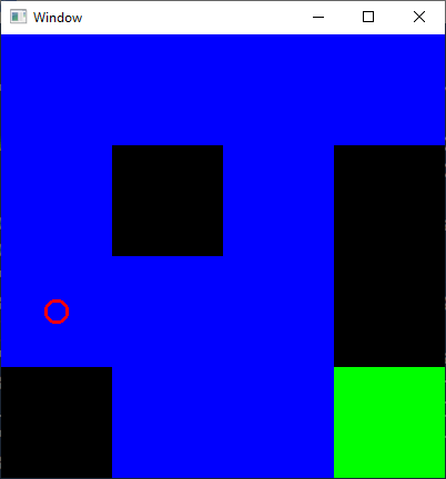
CONCLUSION

With a little more plumbing, it would be possible to combine this with the rest of our "Environment" work. There are some definite challenges. Our current environment setup doesn't have a "time update" function. Combining machine learning with Gloss rendering would also be interesting.

This is the end of the Open AI Gym series, but take a look at our Github repository to see all the code we wrote in this series! The code for this article is on the gloss branch, particularly in FrozenLakeGloss.hs, with some modifications to FrozenLakeBasic.hs. If you liked this series, don't forget to Subscribe to Monday Morning Haskell to get our monthly newsletter!

Parsing with Haskell

Parsing Primer: Gherkin Syntax

Haskell is a truly awesome language for parsing. Haskell expressions tend to compose in simple ways with very clearly controlled side effects. This provides an ideal environment in which to break down parsing into simpler tasks. Thus there are many excellent parsing libraries out there.

In this series, we'll be taking a tour of some of these libraries. But before we look at specific code, it will be useful to establish a common example for what we're going to be parsing. In this first part, I'll introduce Gherkin Syntax, the language behind the Cucumber framework. We'll go through the language specifics, then show the basics of how we set ourselves up for success in Haskell.

If you're already familiar with Gherkin syntax, feel free to move on to part 2 of this series! Or if you want to challenge yourself with more libraries to learn, you can download our Production Checklist. It'll give you a survey of libraries for many different tasks!

Like some of our other series, there's a Github Repository that has all the code for these tutorials! You can observe some Gherkin examples in this directory. We'll compose our Haskell types in this module.

GHERKIN BACKGROUND

Cucumber is a framework for Behavior Driven Development. Under BDD, we first describe all the general behaviors we want our code to perform in plain language. This paradigm is an alternative to Test Driven Development. There, we use test cases to determine our next programming objectives. But BDD can do both of these if we can take behavior descriptions and automatically create tests from them! This would allow less technical members of a project team to effectively write tests!

The main challenge of this is formalizing a language for describing these behaviors. If we have a formal language, then we can parse it. If we can parse it into a reasonable structure, then we can turn that structure into runnable test code. This series will focus on the second part of this problem: turning Gherkin Syntax into a data structure (a Haskell data structure, in our case).

GHERKIN SYNTAX

Gherkin syntax has many complexities, but for these articles we'll be focusing on the core elements of it. The behaviors you want to test are broken down into a series of features. We describe each feature in its own .feature file. So our overarching task is to read input from a single file and turn it into a Feature object.

We begin our description of a feature with the Feature keyword (obviously). We'll give it a title, and then give it an indented description (our example will be a simple banking app):

Feature: Registering a User
  As a potential user
  I want to be able to create an account with a username,
    email and password
  So that I can start depositing money into my account

Each feature then has a series of scenarios. These describe specific cases of what can happen as part of this feature. Each scenario begins with the Scenario keyword and a title.

Scenario: Successful registration
  ...

Scenario: Email is already taken
  ...

Scenario: Username is already taken
  ...

Each scenario then has a series of Gherkin statements. These statements begin with one of the keywords Given, When, Then, or And. You should use Given statements to describe pre-conditions of the scenario. Then you'll use When to describe the particular action a user is taking to initiate the scenario. And finally, you'll use Then to describe the after effects.

Scenario: Email is already taken
  Given there is already an account with the email "test@test.com"
  When I register an account with username "test",
    email "test@test.com" and password "1234abcd!?"
  Then it should fail with an error:
    "An account with that email already exists"
You can supplement any of these cases with a statement beginning with And.

Scenario: Email is already taken
  Given there is already an account with the email "test@test.com"
  And there is already an account with the username "test"
  When I register an account with username "test",
    email "test@test.com" and password "1234abcd!?"
  Then it should fail with an error: 
    "An account with that email already exists"
  And there should still only be one account with 
    the email "test@test.com"

Gherkin syntax does not enforce that you use the different keywords in a semantically sound way. We could start every statement with Given and it would still work. But obviously you should do whatever you can to make your tests sound correct.

We can also fill in statements with variables in angle brackets. We'll then follow the scenario with a table of examples for those variables:

Scenario: Successful Registration
  Given There is no account with username <username>
    or email <email>
  When I register the account with username <username>,
    email <email> and password <password>
  Then it should successfully create the account
    with <username>, <email>, and <password>
  Examples:
    | username | email              | password      |
    | john doe | john@doe.com       | ABCD1234!?    |
    | jane doe | jane.doe@gmail.com | abcdefgh1.aba |
    | jackson  | jackson@yahoo.com  | cadsw4ll0p/   |

We can also create a Background for the whole feature. This is a scenario-like description of preconditions that exist for every scenario in that feature. This can also have an example table:

Feature: User Log In
  ...

Background:
  Given: There is an existing user with username <username>,
    email <email> and password <password>
  Examples:
    | username | email              | password      |
    | john doe | john@doe.com       | ABCD1234!?    |
    | jane doe | jane.doe@gmail.com | abcdefgh1.aba |

And that's the whole language we're going to be working with!

HASKELL DATA STRUCTURES

Let's appreciate now how easy it is to create data structures in Haskell to represent this syntax. We'll start with a description of a Feature. It has a title, description (which we'll treat as a list of multiple lines), the background, and then a list of scenarios. We'll also treat the background like a "nameless" scenario that may or may not exist:

data Feature = Feature
  { featureTitle :: String
  , featureDescription :: [String]
  , featureBackground :: Maybe Scenario
  , featureScenarios :: [Scenario]
  }

Now let's describe what a Scenario is. It's main components are its title and a list of statements. We'll also observe that we should have some kind of structure for the list of examples we'll provide:

data Scenario = Scenario
  { scenarioTitle :: String
  , scenarioStatements :: [Statement]
  , scenarioExamples :: ExampleTable
  }

This ExampleTable will store a list of possible keys as well as list of tuple maps. Each tuple will contain keys and values. At the scale we're likely to be working at, it's not worth it to use a full Map:

data ExampleTable = ExampleTable
  { exampleTableKeys :: [String]
  , exampleTableExamples :: [[(String, Value)]]
  }

Now we'll have to define what we mean by a Value. We'll keep it simple and only use literal bools, strings, numbers, and a null value:

data Value =
  ValueNumber Scientific |
  ValueString String |
  ValueBool Bool |
  ValueNull

And finally we'll describe a statement. This will have the string itself, as well as a list of variable keywords to interpolate:

data Statement = Statement
  { statementText :: String
  , statementExampleVariables :: [String]
  }

And that's all there is too it! We can put all these types in a single file and feel pretty good about that. In Java or C++, we would want to make a separate file (or two!) for each type and there would be a lot more boilerplate involved.

GENERAL PARSING APPROACH

Another reason we'll see that Haskell is good for parsing is the ease of breaking problems down into smaller pieces. We'll have one function for parsing an example table, a different function for parsing a statement, and so on. Then gluing these together will actually be slick and simple!

CONCLUSION

Now you can move on to part 2 where we'll actually look at how to start parsing this. The first library we'll use is the regex-applicative parsing library. We'll see how we can get a lot of what we want without even using a monadic context!

For some more ideas on parsing libraries you can use, check out our free Production Checklist. It will tell you about different libraries for parsing as well as a great many other tasks, from data structures to web APIs!

Applicative Parsing

In part 1 of this series, we prepared ourselves for parsing by going over the basics of the Gherkin Syntax. In this part, we'll be using Regular Expression (Regex) based, applicative parsing to parse the syntax. We'll start by focusing on the fundamentals of this library and building up a vocabulary of combinators to use. We'll make heavy use of the Applicative typeclass. If you need a refresher on that, check out this article.

As we start coding, you can also follow along with the examples on Github here! Most of the code here is in the RegexParser module.

If you're itching to try a monadic approach to parsing, be sure to check out part 3 of this series, where we'll learn about the Attoparsec library. If you want to learn about a wider variety of production utilities, download our Production Checklist. It summarizes many other useful libraries for writing higher level Haskell.

GETTING STARTED

So to start parsing, let's make some notes about our input format. First, we'll treat our input feature document as a single string. We'll remove all empty lines, and then trim leading and trailing whitespace from each line.

parseFeatureFromFile :: FilePath -> IO Feature
parseFeatureFromFile inputFile = do
  fileContents <- lines <$> readFile inputFile
  let nonEmptyLines = filter (not . isEmpty) fileContents
  let trimmedLines = map trim nonEmptyLines
  let finalString = unlines trimmedLines
  case parseFeature finalString of
    ...

...

isEmpty :: String -> Bool
isEmpty = all isSpace

trim :: String -> String
trim input = reverse flippedTrimmed
  where
    trimStart = dropWhile isSpace input
    flipped = reverse trimStart
    flippedTrimmed = dropWhile isSpace flipped

This means a few things for our syntax. First, we don't care about indentation. Second, we ignore extra lines. This means our parsers might allow certain formats we don't want. But that's OK because we're trying to keep things simple.

THE RE TYPE

With applicative based parsing, the main data type we'll be working with is called RE, for regular expression. This represents a parser, and it's parameterized by two types:

data RE s a = ...

The s type refers to the fundamental unit we'll be parsing. Since we're parsing our input as a single String, this will be Char. Then the a type is the result of the parsing element. This varies from parser to parser. The most basic combinator we can use is sym. This parses a single symbol of your choosing:

sym :: s - > RE s s

parseLowercaseA :: RE Char Char
parseLowercaseA = sym 'a'

To use an RE parser, we call the match function or its infix equivalent =~. These will return a Just value if we can match the entire input string, and Nothing otherwise:

>> match parseLowercaseA "a"
Just 'a'
>> "b" =~ parseLowercaseA
Nothing
>> "ab" =~ parseLowercaseA
Nothing -- (Needs to parse entire input)

PREDICATES AND STRINGS

Naturally, we'll want some more complicated functionality. Instead of parsing a single input character, we can parse any character that fits a particular predicate by using psym. So if we want to read any character that was not a newline, we could do:

parseNonNewline :: RE Char Char
parseNonNewline = psym (/= '\n')

The string combinator allows us to match a particular full string and then return it:

readFeatureWord :: RE Char String
readFeatureWord = string "Feature"

We'll use this for parsing keywords, though we'll often end up discarding the "result".

APPLICATIVE COMBINATORS

Now the RE type is applicative. This means we can apply all kinds of applicative combinators over it. One of these is many, which allows us to apply a single parser several times. Here is one combinator that we'll use a lot. It allows us to read everything up until a newline and return the resulting string:

readUntilEndOfLine :: RE Char String
readUntilEndOfLine = many (psym (/= '\n'))

Beyond this, we'll want to make use of the applicative <*> operator to combine different parsers. We can also apply a pure function (or constructor) on top of those by using <$>. Suppose we have a data type that stores two characters. Here's how we can build a parser for it:

data TwoChars = TwoChars Char Char

parseTwoChars :: RE Char TwoChars
parseTwoChars = TwoChars <$> parseNonNewline <*> parseNonNewline

...

>> match parseTwoChars "ab"
Just (TwoChars 'a' 'b')

We can also use <* and *>, which are cousins of the main applicative operator. The first one will parse but then ignore the right hand parse result. The second discards the left side result.

parseFirst :: RE Char Char
parseFirst = parseNonNewline <* parseNonNewline

parseSecond :: RE Char Char
parseSecond = parseNonNewline *> parseNonnewline
>> match parseFirst "ab"
Just 'a'
>> match parseSecond "ab"
Just 'b'
>> match parseFirst "a"
Nothing

Notice the last one fails because the parser needs to have both inputs! We'll come back to this idea of failure in a second. But now that we know this technique, we can write a couple other useful parsers:

readThroughEndOfLine :: RE Char String
readThroughEndOfLine = readUntilEndOfLine <* sym '\n'

readThroughBar :: RE Char String
readThroughBar = readUntilBar <* sym '|'

readUntilBar :: RE Char String
readUntilBar = many (psym (\c -> c /= '|' && c /= '\n'))

The first will parse the rest of the line and then consume the newline character itself. The other parsers accomplish this same task, except with the vertical bar character. We'll need these when we parse the Examples section further down.

ALTERNATIVES: DEALING WITH PARSE FAILURE

We introduced the notion of a parser "failing" up above. Of course, we need to be able to offer alternatives when a parser fails! Otherwise our language will be very limited in its structure. Luckily, the RE type also implements Alternative. This means we can use the <|> operator to determine an alternative parser when one fails. Let's see this in action:

parseFeatureTitle :: RE Char String
parseFeatureTitle = string "Feature: " *> readThroughEndOfLine

parseScenarioTitle :: RE Char String
parseScenarioTitle = string "Scenario: " *> readThroughEndOfLine

parseEither :: RE Char String
parseEither = parseFeatureTitle <|> parseScenarioTitle
>> match parseFeatureTitle "Feature: Login\n"
Just "Login"
>> match parseFeatureTitle "Scenario: Login\n"
Nothing
>> match parseEither "Scenario: Login\n"
Just "Login"

Of course, if ALL the options fail, then we'll still have a failing parser!

>> match parseEither "Random: Login\n"
Nothing

We'll need this to introduce some level of choice into our parsing system. For instance, it's up to the user if they want to include a Background as part of their feature. So we need to be able to read the background if it's there or else move onto parsing a scenario.

VALUE PARSER

In keeping with our approach from the last article, we're going to start with smaller elements of our syntax. Then we can use these to build larger ones with ease. To that end, let's build a parser for our Value type, the most basic data structure in our syntax. Let's recall what that looks like:

data Value =
  ValueNull |
  ValueBool Bool |
  ValueString String |
  ValueNumber Scientific

Since we have different constructors, we'll make a parser for each one. Then we can combine them with alternative syntax:

valueParser :: RE Char Value
valueParser =
  nullParser <|>
  boolParser <|>
  numberParser <|>
  stringParser

Now our parsers for the null values and boolean values are easy. For each of them, we'll give a few different options about what strings we can use to represent those elements. Then, as with the larger parser, we'll combine them with <|>.

nullParser :: RE Char Value
nullParser =
  (string "null" <|>
  string "NULL" <|>
  string "Null") *> pure ValueNull

boolParser :: RE Char Value
boolParser =
  trueParser *> pure (ValueBool True) <|> 
  falseParser *> pure (ValueBool False)
  where
    trueParser = string "True" <|> string "true" <|> string "TRUE"
    falseParser = string "False" <|> string "false" <|> string "FALSE"
```haskell
Notice in both these cases we discard the actual string with *> and then return our constructor. We have to wrap the desired result with pure.

# NUMBER AND STRING VALUES
Numbers and strings are a little more complicated since we can't rely on hard-coded formats. In the case of numbers, we'll account for integers, decimals, and negative numbers. We'll ignore scientific notation for now. An integer is simple to parse, since we'll have many characters that are all numbers. We use some instead of many to enforce that there is at least one:
```haskell
numberParser :: RE Char Value
numberPaser = ...
  where
    integerParser = some (psym isNumber)

A decimal parser will read some numbers, then a decimal point, and then more numbers. We'll insist there is at least one number after the decimal point.

numberParser :: RE Char Value
numberPaser = ...
  where
    integerParser = some (psym isNumber)
    decimalParser = 
      many (psym isNumber) <*> sym '.' <*> some (psym isNumber)

Finally, for negative numbers, we'll read a negative symbol and then one of the other parsers:

numberParser :: RE Char Value
numberPaser = ...
  where
    integerParser = some (psym isNumber)
    decimalParser = 
      many (psym isNumber) <*> sym '.' <*> some (psym isNumber)
    negativeParser = sym '-' <*> (decimalParser <|> integerParser)

However, we can't combine these parsers as is! Right now, they all return different results! The integer parser returns a single string. The decimal parser returns two strings and the decimal character, and so on. In general, we'll want to combine each parser's results into a single string and then pass them to the read function. This requires mapping a couple functions over our last two parsers:

numberParser :: RE Char Value
numberPaser = ...
  where
    integerParser = some (psym isNumber)
    decimalParser = combineDecimal <$> 
      many (psym isNumber) <*> sym '.' <*> some (psym isNumber)
    negativeParser = (:) <$> 
      sym '-' <*> (decimalParser <|> integerParser)

    combineDecimal :: String -> Char -> String -> String
    combineDecimal base point decimal = base ++ (point : decimal)

Now all our number parsers return strings, so we can safely combine them. We'll map the ValueNumber constructor over the value we read from the string.

numberParser :: RE Char Value
numberPaser = (ValueNumber . read) <$>
  (negativeParser <|> decimalParser <|> integerParser)
  where
    ...

Note that order matters! If we put the integer parser first, we'll be in trouble! If we encounter a decimal, the integer parser will greedily succeed and parse everything before the decimal point. We'll either lose all the information after the decimal, or worse, have a parse failure.

The last thing we need to do is read a string. We need to read everything in the example cell until we hit a vertical bar, but then ignore any whitespace. Luckily, we have the right combinator for this, and we've even written a trim function already!

stringParser :: RE Char Value
stringParser = (ValueString . trim) <$> readUntilBar

And now our valueParser will work as expected!

BUILDING AN EXAMPLE TABLE

Now that we can parse individual values, let's figure out how to parse the full example table. We can use our individual value parser to parse a whole line of values! The first step is to read the vertical bar at the start of the line.

exampleLineParser :: RE Char [Value]
exampleLineParser = sym '|' *> ...

Next, we'll build a parser for each cell. It will read the whitespace, then the value, and then read up through the next bar.

exampleLineParser :: RE Char [Value]
exampleLineParser = sym '|' *> ...
  where
    cellParser = 
      many isNonNewlineSpace *> valueParser <* readThroughBar

isNonNewlineSpace :: RE Char Char
isNonNewlineSpace = psym (\c -> isSpace c && c /= '\n')

Now we read many of these and finish by reading the newline:

exampleLineParser :: RE Char [Value]
exampleLineParser = 
  sym '|' *> many cellParser <* readThroughEndOfLine
  where
    cellParser = 
      many isNonNewlineSpace *> valueParser <* readThroughBar

Now, we need a similar parser that reads the title column of our examples. This will have the same structure as the value cells, only it will read normal alphabetic strings instead of values.

exampleColumnTitleLineParser :: RE Char [String]
exampleColumnTitleLineParser = sym '|' *> many cellParser <* readThroughEndOfLine
  where
    cellParser = 
      many isNonNewlineSpace *> many (psym isAlpha) <* readThroughBar

Now we can start building the full example parser. We'll want to read the string, the column titles, and then the value lines.

exampleTableParser :: RE Char ExampleTable
exampleTableParser =
  (string "Examples:" *> readThroughEndOfLine) *>
  exampleColumnTitleLineParser <*>
  many exampleLineParser
``
We're not quite done yet. We'll need to apply a function over these results that will produce the final ExampleTable. And the trick is that we want to map up the example keys with their values. We can accomplish this with a simple function. It will return zip the keys over each value list using map:
```haskell
exampleTableParser :: RE Char ExampleTable
exampleTableParser = buildExampleTable <$>
  (string "Examples:" *> readThroughEndOfLine) *>
  exampleColumnTitleLineParser <*>
  many exampleLineParser
  where
    buildExampleTable :: [String] -> [[Value]] -> ExampleTable
    buildExampleTable keys valueLists = ExampleTable keys (map (zip keys) valueLists)

STATEMENTS

Now we that we can parse the examples for a given scenario, we need to parse the Gherkin statements. To start with, let's make a generic parser that takes the keyword as an argument. Then our full parser will try each of the different statement keywords:

parseStatementLine :: String -> RE Char Statement
parseStatementLine signal = ...

parseStatement :: RE Char Statement
parseStatement =
  parseStatementLine "Given" <|>
  parseStatementLine "When" <|>
  parseStatementLine "Then" <|>
  parseStatementLine "And"

Now we'll get the signal word out of the way and parse the statement line itself.

parseStatementLine :: String -> RE Char Statement
parseStatementLine signal = string signal *> sym ' ' *> ...

Parsing the statement is tricky. We want to parse the keys inside brackets and separate them as keys. But we also want them as part of the statement's string. To that end, we'll make two helper parsers. First, nonBrackets will parse everything in a string up through a bracket (or a newline).

nonBrackets :: RE Char String
nonBrackets = many (psym (\c -> c /= '\n' && c /= '<'))

We'll also want a parser that parses the brackets and returns the keyword inside:

insideBrackets :: RE Char String
insideBrackets = sym '<' *> many (psym (/= '>')) <* sym '>'

Now to read a statement, we start with non-brackets, and alternate with keys in brackets. Let's observe that we start and end with non-brackets, since they can be empty. Thus we can represent a line a list of non-bracket/bracket pairs, followed by a last non-bracket part. To make a pair, we combine the parser results in a tuple using the (,) constructor enabled by TupleSections:

parseStatementLine :: String -> RE Char Statement
parseStatementLine signal = string signal *> sym ' ' *>
  many ((,) <$> nonBrackets <*> insideBrackets) <*> nonBrackets

From here, we need a recursive function that will build up our final statement string and the list of keys. We do this with buildStatement.

parseStatementLine :: String -> RE Char Statement
parseStatementLine signal = string signal *> sym ' ' *>
  (buildStatement <$> 
    many ((,) <$> nonBrackets <*> insideBrackets) <*> nonBrackets)
  where
    buildStatement :: 
      [(String, String)] -> String -> (String, [String])
    buildStatement [] last = (last, [])
    buildStatement ((str, key) : rest) rem =
      let (str', keys) = buildStatement rest rem
      in (str <> "<" <> key <> ">" <> str', key : keys)

The last thing we need is a final helper that will take the result of buildStatement and turn it into a Statement. We'll call this finalizeStatement, and then we're done!

parseStatementLine :: String -> RE Char Statement
parseStatementLine signal = string signal *> sym ' ' *>
  (finalizeStatement . buildStatement <$> 
    many ((,) <$> nonBrackets <*> insideBrackets) <*> nonBrackets)
  where
    buildStatement :: 
      [(String, String)] -> String -> (String, [String])
    buildStatement [] last = (last, [])
    buildStatement ((str, key) : rest) rem =
      let (str', keys) = buildStatement rest rem
      in (str <> "<" <> key <> ">" <> str', key : keys)

    finalizeStatement :: (String, [String]) -> Statement
    finalizeStatement (regex, variables) = Statement regex variables

SCENARIOS

Now that we have all our pieces in place, it's quite easy to write the parser for scenario! First we get the title by reading the keyword and then the rest of the line:

scenarioParser :: RE Char Scenario
scenarioParser = string "Scenario: " *> readThroughEndOfLine ...

After that, we read many statements, and then the example table. Since the example table might not exist, we'll provide an alternative that is a pure, empty table. We can wrap everything together by mapping the Scenario constructor over it.

scenarioParser :: RE Char Scenario
scenarioParser = Scenario <$>
  (string "Scenario: " *> readThroughEndOfLine) <*>
  many (statementParser <* sym '\n') <*>
  (exampleTableParser <|> pure (ExampleTable [] []))

We can also make a "Background" parser that is very similar. All that changes is that we read the string "Background" instead of a title. Since we'll hard-code the title as "Background", we can include it with the constructor and map it over the parser.

backgroundParser :: RE Char Scenario
backgroundParser = Scenario "Background" <$>
  (string "Background:" *> readThroughEndOfLine) *>
 many (statementParser <* sym '\n') <*>
  (exampleTableParser <|> pure (ExampleTable [] []))

FINALLY THE FEATURE

We're almost done! All we have left is to write the featureParser itself! As with scenarios, we'll start with the keyword and a title line:

featureParser :: RE Char Feature
featureParser = Feature <$>
  (string "Feature: " *> readThroughEndOfLine) <*>
  ...

Now we'll use the optional combinator to parse the Background if it exists, but return Nothing if it doesn't. Then we'll wrap up with parsing many scenarios!

featureParser :: RE Char Feature
featureParser = Feature <$>
  (string "Feature: " *> readThroughEndOfLine) <*>
  pure [] <*>
  (optional backgroundParser) <*>
  (many scenarioParser)

Note that here we're ignoring the "description" of a feature we proposed as part of our original syntax and simply giving an empty list of strings. Since there are no keywords for that, it turns out to be painful to deal with it using applicative parsing. When we look at monadic approaches starting next week, we'll see it isn't as hard there.

CONCLUSION

This wraps up our exploration of applicative parsing. We can see how well suited Haskell is for parsing. The functional nature of the language means it's easy to start with small building blocks like our first parsers. Then we can gradually combine them to make something larger. It can be a little tricky to wrap our heads around all the different operators and combinators. But once you understand the ways in which these let us combine our parsers, they make a lot of sense and are easy to use.

You should now move onto part 3 of this series, where we will start learning about monadic parsing. You'll get to see how we use the Attoparsec library to parse this same Gherkin syntax!

To further your knowledge of useful Haskell libraries, download our free Production Checklist! It will tell you about libraries for many tasks, from databases to machine learning!

If you've never written a line of Haskell before, never fear! Download our Beginners Checklist to learn more!

Attoparsec

In part 2 of this series we looked at the Regex-based Applicative Parsing library. We took a lot of smaller combinators and put them together to parse our Gherkin syntax (check out part 1 for a quick refresher on that).

This week, we'll look at a new library: Attoparsec. Instead of trying to do everything with a purely applicative structure, this library uses a monadic approach. This approach is much more common. It results in syntax that is simpler to read and understand. It will also make it easier for us to add certain features.

To follow along with the code for this article, take a look at the AttoParser module on Github! For some more excellent ideas about useful libraries, download our Production Checklist! It includes material on libraries for everything from data structures to machine learning!

Finally, if you already know about Attoparsec, feel free to move onto part 4 and learn about Megaparsec!

THE PARSER TYPE

In applicative parsing, all our parsers had the type RE Char. This type belonged to the Applicative typeclass but was not a Monad. For Attoparsec, we'll instead be using the Parser type, a full monad. So in general we'll be writing parsers with the following types:

featureParser :: Parser Feature
scenarioParser :: Parser Scenario
statementParser :: Parser Statement
exampleTableParser :: Parser ExampleTable
valueParser :: Parser Value

PARSING VALUES

The first thing we should realize though is that our parser is still an Applicative! So not everything needs to change! We can still make use of operators like *> and <|>. In fact, we can leave our value parsing code almost exactly the same! For instance, the valueParser, nullParser, and boolParser expressions can remain the same:

valueParser :: Parser Value
valueParser =
  nullParser <|>
  boolParser <|>
  numberParser <|>
  stringParser

nullParser :: Parser Value
nullParser =
  (string "null" <|>
  string "NULL" <|>
  string "Null") *> pure ValueNull

boolParser :: Parser Value
boolParser = (trueParser *> pure (ValueBool True)) <|> (falseParser *> pure (ValueBool False))
  where
    trueParser = string "True" <|> string "true" <|> string "TRUE"
    falseParser = string "False" <|> string "false" <|> string "FALSE"

If we wanted, we could make these more "monadic" without changing their structure. For instance, we can use return instead of pure (since they are identical). We can also use >> instead of *> to perform monadic actions while discarding a result. Our value parser for numbers changes a bit, but it gets simpler! The authors of Attoparsec provide a convenient parser for reading scientific numbers:

numberParser :: Parser Value
numberParser = ValueNumber <$> scientific

Then for string values, we'll use the takeTill combinator to read all the characters until a vertical bar or newline. Then we'll apply a few text functions to remove the whitespace and get it back to a String. (The Parser monad we're using parses things as Text rather than String).

stringParser :: Parser Value
stringParser = (ValueString . unpack . strip) <$> 
  takeTill (\c -> c == '|' || c == '\n')

PARSING EXAMPLES

As we parse the example table, we'll switch to a more monadic approach by using do-syntax. First, we establish a cellParser that will read a value within a cell.

cellParser = do
  skipWhile nonNewlineSpace
  val <- valueParser
  skipWhile (not . barOrNewline)
  char '|'
  return val

Each line in our statement refers to a step of the parsing process. So first we skip all the leading whitespace. Then we parse our value. Then we skip the remaining space, and parse the final vertical bar to end the cell. Then we'll return the value we parsed.

It's a lot easier to keep track of what's going on here compared to applicative syntax. It's not hard to see which parts of the input we discard and which we use. If we don't assign the value with <- within do-syntax, we discard the value. If we retrieve it, we'll use it. To complete the exampleLineParser, we parse the initial bar, get many values, close out the line, and then return them:

exampleLineParser :: Parser [Value]
exampleLineParser = do
  char '|'
  cells <- many cellParser
  char '\n'
  return cells
  where
    cellParser = ...

Reading the keys for the table is almost identical. All that changes is that our cellParser uses many letter instead of valueParser. So now we can put these pieces together for our exampleTableParser:

exampleTableParser :: Parser ExampleTable
exampleTableParser = do
  string "Examples:"
  consumeLine
  keys <- exampleColumnTitleLineParser
  valueLists <- many exampleLineParser
  return $ ExampleTable keys (map (zip keys) valueLists)

We read the signal string "Examples:", followed by consuming the line. Then we get our keys and values, and build the table with them. Again, this is much simpler than mapping a function like buildExampleTable like in applicative syntax.

STATEMENTS

The Statement parser is another area where we can improve the clarity of our code. Once again, we'll define two helper parsers. These will fetch the portions outside brackets and then inside brackets, respectively:

nonBrackets :: Parser String
nonBrackets = many (satisfy (\c -> c /= '\n' && c /= '<'))

insideBrackets :: Parser String
insideBrackets = do
  char '<'
  key <- many letter
  char '>'
  return key

Now when we put these together, we can more clearly see the steps of the process outlined in do-syntax. First we parse the “signal” word, then a space. Then we get the “pairs” of non-bracketed and bracketed portions. Finally, we'll get one last non-bracketed part:

parseStatementLine :: Text -> Parser Statement
parseStatementLine signal = do
  string signal
  char ' '
  pairs <- many ((,) <$> nonBrackets <*> insideBrackets)
  finalString <- nonBrackets
  ...

Now we can define our helper function buildStatement and call it on its own line in do-syntax. Then we'll return the resulting Statement. This is much easier to read than tracking which functions we map over which sections of the parser:

parseStatementLine :: Text -> Parser Statement
parseStatementLine signal = do
  string signal
  char ' '
  pairs <- many ((,) <$> nonBrackets <*> insideBrackets)
  finalString <- nonBrackets
  let (fullString, keys) = buildStatement pairs finalString
  return $ Statement fullString keys
  where
    buildStatement 
      :: [(String, String)] -> String -> (String, [String])
    buildStatement [] last = (last, [])
    buildStatement ((str, key) : rest) rem =
      let (str', keys) = buildStatement rest rem
      in (str <> "<" <> key <> ">" <> str', key : keys)

SCENARIOS AND FEATURES

As with applicative parsing, it's now straightforward for us to finish everything off. To parse a scenario, we read the keyword, consume the line to read the title, and read the statements and examples:

scenarioParser :: Parser Scenario
scenarioParser = do
  string "Scenario: "
  title <- consumeLine
  statements <- many (parseStatement <* char '\n')
  examples <- (exampleTableParser <|> return (ExampleTable [] []))
  return $ Scenario title statements examples

Again, we provide an empty ExampleTable as an alternative if there are no examples. The parser for Background looks very similar. The only difference is we ignore the result of the line and instead use Background as the title string.

backgroundParser :: Parser Scenario
backgroundParser = do
  string "Background:"
  consumeLine
  statements <- many (parseStatement <* char '\n')
  examples <- (exampleTableParser <|> return (ExampleTable [] []))
  return $ Scenario "Background" statements examples

Finally, we'll put all this together as a feature. We read the title, get the background if it exists, and read our scenarios:

featureParser :: Parser Feature
featureParser = do
  string "Feature: "
  title <- consumeLine
  maybeBackground <- optional backgroundParser
  scenarios <- many scenarioParser
  return $ Feature title maybeBackground scenarios

FEATURE DESCRIPTION

One extra feature we'll add now is that we can more easily parse the “description” of a feature. We omitted them in applicative parsing, as it's a real pain to implement. It becomes much simpler when using a monadic approach. The first step we have to take though is to make one parser for all the main elements of our feature. This approach looks like this:

featureParser :: Parser Feature
featureParser = do
  string "Feature: "
  title <- consumeLine
  (description, maybeBackground, scenarios) <- parseRestOfFeature
  return $ Feature title description maybeBackground scenarios

parseRestOfFeature :: Parser ([String], Maybe Scenario, [Scenario])
parseRestOfFeature = ...

Now we'll use a recursive function that reads one line of the description at a time and adds to a growing list. The trick is that we'll use the choice combinator offered by Attoparsec.

We'll create two parsers. The first assumes there are no further lines of description. It attempts to parse the background and scenario list. The second reads a line of description, adds it to our growing list, and recurses:

parseRestOfFeature :: Parser ([String], Maybe Scenario, [Scenario])
parseRestOfFeature = parseRestOfFeatureTail []
  where
    parseRestOfFeatureTail prevDesc = do
      (fullDesc, maybeBG, scenarios) <- choice [noDescriptionLine prevDesc, descriptionLine prevDesc]
      return (fullDesc, maybeBG, scenarios)

So we'll first try to run this noDescriptionLineParser. It will try to read the background and then the scenarios as we've always done. If it succeeds, we know we're done. The argument we passed is the full description:

where
  noDescriptionLine prevDesc = do
    maybeBackground <- optional backgroundParser
    scenarios <- some scenarioParser
    return (prevDesc, maybeBackground, scenarios)

Now if this parser fails, we know that it means the next line is actually part of the description. So we'll write a parser to consume a full line, and then recurse:

descriptionLine prevDesc = do
  nextLine <- consumeLine
  parseRestOfFeatureTail (prevDesc ++ [nextLine])

And now we're done! We can parse descriptions!

CONCLUSION

That wraps up our exploration of Attoparsec. Now you can move on to the fourth and final part of this series where we'll learn about Megaparsec. We'll find that it's syntactically very similar to Attoparsec with a few small exceptions. We'll see how we can use some of the added power of monadic parsing to enrich our syntax.

To learn more about cool Haskell libraries, be sure to check out our Production Checklist! It'll tell you a little bit about libraries in all kinds of areas like databases and web APIs.

If you've never written Haskell at all, download our Beginner's Checklist! It'll give you all the resources you need to get started on your Haskell journey!

Megaparsec

In part 3 of this series, we explored the Attoparsec library. It provided us with a clearer syntax to work with compared to applicative parsing, which we learned in part 2. This week, we'll explore one final library: Megaparsec.

This library has a lot in common with Attoparsec. In fact, the two have a lot of compatibility by design. Ultimately, we'll find that we don't need to change our syntax a whole lot. But Megaparsec does have a few extra features that can make our lives simpler.

To follow the code examples here, head to the Github repository and take a look at the MegaParser module on Github! To learn about more awesome libraries you can use in production, make sure to download our Production Checklist! But never fear if you're new to Haskell! Just take a look at our Beginners checklist and you'll know where to get started!

A DIFFERENT PARSER TYPE

To start out, the basic parsing type for Megaparsec is a little more complicated. It has two type parameters, e and s, and also comes with a built-in monad transformer ParsecT.

data ParsecT e s m a = ParsecT ...

type Parsec e s = ParsecT e s Identity

The e type allows us to provide some custom error data to our parser. The s type refers to the input type of our parser, typically some variant of String. This parameter also exists under the hood in Attoparsec. But we sidestepped that issue by using the Text module. For now, we'll set up our own type alias that will sweep these parameters under the rug:

type MParser = Parsec Void Text

TRYING OUR HARDEST

Let's start filling in our parsers. There's one structural difference between Attoparsec and Megaparsec. When a parser fails in Attoparsec, its default behavior is to backtrack. This means it acts as though it consumed no input. This is not the case in Megaparsec! A naive attempt to repeat our nullParser code could fail in some ways:

nullParser :: MParser Value
nullParser = nullWordParser >> return ValueNull
  where
    nullWordParser = string "Null" <|> string "NULL" <|> string "null"

Suppose we get the input "NULL" for this parser. Our program will attempt to select the first parser, which will parse the N token. Then it will fail on U. It will move on to the second parser, but it will have already consumed the N! Thus the second and third parser will both fail as well!

We get around this issue by using the try combinator. Using try gives us the Attoparsec behavior of backtracking if our parser fails. The following will work without issue:

nullParser :: MParser Value
nullParser = nullWordParser >> return ValueNull
  where
    nullWordParser = 
      try (string "Null") <|>
      try (string "NULL") <|>
      try (string "null")

Even better, Megaparsec also has a convenience function string' for case insensitive parsing. So our null and boolean parsers become even simpler:

nullParser :: MParser Value
nullParser = M.string' "null" >> return ValueNull

boolParser :: MParser Value
boolParser = 
  (trueParser >> return (ValueBool True)) <|> 
  (falseParser >> return (ValueBool False))
    where
      trueParser = M.string' "true"
      falseParser = M.string' "false"

Unlike Attoparsec, we don't have a convenient parser for scientific numbers. We'll have to go back to our logic from applicative parsing, only this time with monadic syntax.

numberParser :: MParser Value
numberParser = (ValueNumber . read) <$>
  (negativeParser <|> decimalParser <|> integerParser)
  where
    integerParser :: MParser String
    integerParser = M.try (some M.digitChar)

    decimalParser :: MParser String
    decimalParser = M.try $ do
      front <- many M.digitChar
      M.char '.'
      back <- some M.digitChar
      return $ front ++ ('.' : back)

    negativeParser :: MParser String
    negativeParser = M.try $ do
      M.char '-'
      num <- decimalParser <|> integerParser
      return $ '-' : num

Notice that each of our first two parsers use try to allow proper backtracking. For parsing strings, we'll use the satisfy combinator to read everything up until a bar or newline:

stringParser :: MParser Value
stringParser = (ValueString . trim) <$>
  many (M.satisfy (not . barOrNewline))

And then filling in our value parser is easy as it was before:

valueParser :: MParser Value
valueParser =
  nullParser <|>
  boolParser <|>
  numberParser <|>
  stringParser

FILLING IN THE DETAILS

Aside from some trivial alterations, nothing changes about how we parse example tables. The Statement parser requires adding in another try call when we're grabbing our pairs:

parseStatementLine :: Text -> MParser Statement
parseStatementLine signal = do
  M.string signal
  M.char ' '
  pairs <- many $ M.try ((,) <$> nonBrackets <*> insideBrackets)
  finalString <- nonBrackets
  let (fullString, keys) = buildStatement pairs finalString
  return $ Statement fullString keys
  where
    buildStatement  = ...

Otherwise, we'll fail on any case where we don't use any keywords in the statement! But it's otherwise the same. Of course, we also need to change how we call our parser in the first place. We'll use the runParser function instead of Attoparsec's parseOnly. This takes an extra argument for the source file of our parser to provide better messages.

parseFeatureFromFile :: FilePath -> IO Feature
parseFeatureFromFile inputFile = do
  ...
  case runParser featureParser finalString inputFile of
    Left s -> error (show s)
    Right feature -> return feature

But nothing else changes in the structure of our parsers. It's very easy to take Attoparsec code and Megaparsec code and re-use it with the other library!

ADDING SOME STATE

One bonus we do get from Megaparsec is that its monad transformer makes it easier for us to use other monadic functionality. Our parser for statement lines has always been a little bit clunky. Let's clean it up a little bit by allowing ourselves to store a list of strings as a state object. Here's how we'll change our parser type:

type MParser = ParsecT Void Text (State [String])

Now whenever we parse a key using our brackets parser, we can append that key to our existing list using modify. We'll also return the brackets along with the string instead of merely the keyword:

insideBrackets :: MParser String
insideBrackets = do
  M.char '<'
  key <- many M.letterChar
  M.char '>'
  modify (++ [key]) -- Store the key in the state!
  return $ ('<' : key) ++ ['>']

Now instead of forming tuples, we can concatenate the strings we parse!

parseStatementLine :: Text -> MParser Statement
parseStatementLine signal = do
  M.string signal
  M.char ' '
  pairs <- many $ M.try ((++) <$> nonBrackets <*> insideBrackets)
  finalString <- nonBrackets
  let fullString = concat pairs ++ finalString
  ...

And now how do we get our final list of keys? Simple! We get our state value, reset it, and return everything. No need for our messy buildStatement function!

parseStatementLine :: Text -> MParser Statement
parseStatementLine signal = do
  M.string signal
  M.char ' '
  pairs <- many $ M.try ((++) <$> nonBrackets <*> insideBrackets)
  finalString <- nonBrackets
  let fullString = concat pairs ++ finalString
  keys <- get
  put []
  return $ Statement fullString keys

When we run this parser at the start, we now have to use runParserT instead of runParser. This returns us an action in the State monad, meaning we have to use evalState to get our final result:

parseFeatureFromFile :: FilePath -> IO Feature
parseFeatureFromFile inputFile = do
  ...
  case evalState (stateAction finalString) [] of
    Left s -> error (show s)
    Right feature -> return feature
  where
    stateAction s = runParserT featureParser inputFile s

BONUSES OF MEGAPARSEC

As a last bonus, let's look at error messages in Megaparsec. When we have errors in Attoparsec, the parseOnly function gives us an error string. But it's not that helpful. All it tells us is what individual parser on the inside of our system failed:

>> parseOnly nullParser "true"
Left "string"
>> parseOnly "numberParser" "hello"
Left "Failed reading: takeWhile1"

These messages don't tell us where within the input it failed, or what we expected instead. Let's compare this to Megaparsec and runParser:

>> runParser nullParser "true" ""
Left (TrivialError 
  (SourcePos {sourceName = "true", sourceLine = Pos 1, sourceColumn = Pos 1} :| []) 
  (Just EndOfInput) 
  (fromList [Tokens ('n' :| "ull")]))
>> runParser numberParser "hello" ""
Left (TrivialError 
  (SourcePos {sourceName = "hello", sourceLine = Pos 1, sourceColumn = Pos 1} :| []) 
    (Just EndOfInput) 
    (fromList [Tokens ('-' :| ""),Tokens ('.' :| ""),Label ('d' :| "igit")]))

This gives us a lot more information! We can see the string we're trying to parse. We can also see the exact position it fails at. It'll even give us a picture of what parsers it was trying to use. In a larger system, this makes a big difference. We can track down where we've gone wrong either in developing our syntax, or conforming our input to meet the syntax. If we customize the e parameter type, we can even add our own details into the error message to help even more!

CONCLUSION

This wraps up our exploration of parsing libraries in Haskell! In the past few weeks, we've learned about Applicative parsing, Attoparsec, and Megaparsec. The first provides useful and intuitive combinators for when our language is regular. It allows us to avoid using a monad for parsing and the baggage that might bring. With Attoparsec, we saw an introduction to monadic style parsing. This provided us with a syntax that was easier to understand and where we could see what was happening. Finally in this part, we explored Megaparsec. This library has a lot in common syntactically with Attoparsec. But it provides a few more bells and whistles that can make many tasks easier.

Ready to explore some more areas of Haskell development? Want to get some ideas for new libraries to learn? Download our Production Checklist! It'll give you a quick summary of some tools in areas ranging from data structures to web APIs!

Never programmed in Haskell before? Want to get started? Check out our Beginners Checklist! It has all the tools you need to start your Haskell journey!

Haskell API Integrations

Twilio and Text Messages

Welcome to part 1 of our series on Haskell API integrations! Writing our own Haskell code using only simple libraries is fun. But we can't do everything from scratch. There are all kinds of cools services out there to use so we don't have to. We can interface with a lot of these by using APIs. Often, the most well supported APIs use languages like Python and Javascript. But adventurous Haskell developers have also developed bindings for these systems! So in this series, we'll explore a couple of these. We'll also see how to develop our own integration in case one isn't available for the service we want.

In this first part, we'll focus on the Twilio API. We'll see how we can send SMS messages from our Haskell code using the twilio library. We'll also write a simple server to use Twilio's callback system to receive text messages and process them programmatically. You can follow along with the code here on the Github repository for this series. You can find the code for this part in two modules: the SMS module, which has re-usable SMS functions, and the SMSServer module, which has the Servant related code. If you're already familiar with the Haskell Twilio library, you can move onto part 2 where we discuss sending emails with Mailgun!

Of course, none of this is useful if you've never written any Haskell before! If you want to get started with the language basics, download our Beginners Checklist. To learn more about advanced techniques and libraries, grab our Production Checklist!

SETTING UP OUR ACCOUNT

Naturally, you'll need a Twilio account to use the Twilio API. Once you have this set up, you need to add your first Twilio number. This will be the number you'll send text messages to. You'll also see it as the sender for other messages in your system. You should also go through the process of verifying your own phone number. This will allow you to send and receive messages on that phone without "publishing" your app.

You also need a couple other pieces of information from your account. There's the account SID, and the authentication token. You can find these on the dashboard for your project on the Twilio page. You'll need these values in your code. But since you don't want to put them into version control, you should save them as environment variables on your machine. Then when you need to, you can fetch them like so:

fetchSid :: IO String
fetchSid = getEnv "TWILIO_ACCOUT_SID"

fetchToken :: IO String
fetchToken = getEnv "TWILIO_AUTH_TOKEN"

In addition, you should get a Twilio number for your account to send messages from (this might cost a dollar or so). For testing purposes, you should also verify your own phone number on the account dashboard so you can receive messages. Save these as environment variables as well.

import Data.Text (pack)

fetchTwilioNumber :: IO Text 
fetchTwilioNumber = pack <$> getEnv "TWILIO_PHONE_NUMBER"

fetchUserNumber :: IO Text
fetchUserNumber = pack <$> getEnv "TWILIO_USER_NUMBER"

SENDING A MESSAGE

The first thing we'll want to do is use the API to actually send a text message. We perform Twilio actions within the Twilio monad. It's rather straightforward to access this monad from IO. All we need is the runTwilio' function:

runTwilio' :: IO String -> IO String -> Twilio a -> IO a

The first two parameters to this function are IO actions to fetch the account SID and auth token like we have above. Then the final parameter of course is our Twilio action.

sendBasicMessage :: IO ()
sendBasicMessage = runTwilio' fetchSid fetchToken $ do
  ...

To compose a message, we'll use the PostMessage constructor. This takes four parameters. First, the "to" number of our message. Fill this in with the number to your physical phone. Then the second parameter is the "from" number, which has to be our Twilio account's phone number. Then the third parameter is the message itself. The fourth parameter is optional, we can leave it as Maybe. To send the message, all we have to do is use the post function! That's all there is to it!

sendBasicMessage :: IO ()
sendBasicMessage = do
  toNumber <- fetchUserNumber
  fromNumber <- fetchTwilioNumber
  runTwilio' fetchSid fetchToken $ do
    let msg = PostMessage toNumber fromNumber "Hello Twilio!"
    _ <- post msg
    return ()

And just like that, you've sent your first Twilio message! You can just run this IO function from GHCI, and it will send you a text message as long as everything is set up with your Twilio account! Note that it does cost a small amount of money to send messages over Twilio. But a trial account should give you enough free credit to experiment a little bit (as well as cover the initial number).

RECEIVING MESSAGES

Now, it's a little more complicated to deal with incoming messages. First, you need a web server running on the internet. For basic projects like this, I tend to rely on Heroku. If you fork our Github repo, you can easily turn it into your own Heroku server! Just take a look at these instructions in our repo!

The first thing we need to do is create a webhook on our Twilio account. To do this, go to "Manage Numbers" from your project dashboard page (Try this link if you can't find it). Then select your Twilio number. You'll now want to scroll to the section called "Messaging" and then within that, find "A Message Comes In". You want to select "Webhook" in the dropdown. Then you'll need to specify a URL where your server is located, and select "HTTP Post". You can see in this screenshot that we're using my Heroku server with the endpoint path /api/sms.

With this webhook set up, Twilio will send a post request to the endpoint every time a user texts our number. The request will contain the message and the number of the sender. So let's set up a server using Servant to pick up that request.

We'll start by specifying a simple type to encode the message we'll receive from Twilio:

data IncomingMessage = IncomingMessage
  { fromNumber :: Text
  , body :: Text
  }

Twilio encodes its post request body as FormURLEncoded. In order for Servant to deserialize this, we'll need to define an instance of the FromForm class for our type. This function takes in a hash map from keys to lists of values. It will return either an error string or our desired value.

instance FromForm IncomingMessage where
  fromForm :: Form -> Either Text IncomingMessage
  fromForm (From form) = ...

So form is a hash map, and we want to look up the "From" number of the message as well as its body. Then as long as we find at least one result for each of these, we'll return the message. Otherwise, we return an error.

instance FromForm IncomingMessage where
  fromForm :: Form -> Either Text IncomingMessage
  fromForm (From form) = case lookupResults of
    Just ((fromNumber : _), (body : _)) -> 
      Right $ IncomingMessage fromNumber body
    Just _ -> Left "Found the keys but no values"
    Nothing -> Left "Didn't find keys"
    where
      lookupResults = do
        fromNumber <- HashMap.lookup "From" form
        body <- HashMap.lookup "Body" form
        return (fromNumber, body)

Now that we have this instance, we can finally define our API endpoint! All it needs are the simple path components and the request body. For now, we won't actually post any response.

type SMSServerAPI =
  "api" :> "sms" :> ReqBody '[FormUrlEncoded] IncomingMessage :> Post '[JSON] ()

WRITING OUR HANDLER Now let's we want to write a handler for our endpoint that will echo the user's message back to them.

incomingHandler :: IncomingMessage -> Handler ()
incomingHandler (IncomingMessage from body) = liftIO $ do
  twilioNum <- fetchTwilioNumber
  runTwilio' fetchSid fetchToken $ do
    let newMessage = PostMessage from twilioNum body Nothing
    _ <- post newMessage
    return ()

We'll also add an extra endpoint to "ping" our server, just so it's easier to verify that the server is working at a basic level. It will return the string "Pong" to signify the request has been received.

type SMSServerAPI =
  "api" :> "sms" :> ReqBody '[FormUrlEncoded] IncomingMessage :> Post '[JSON] () :<|>
  "api" :> "ping" :> Get '[JSON] String

pingHandler :: Handler String
pingHandler = return "Pong"

And now we wrap up with some of the Servant mechanics to run our server.

smsServerAPI :: Proxy SMSServerAPI
smsServerAPI = Proxy :: Proxy SMSServerAPI

smsServer :: Server SMSServerAPI
smsServer = incomingHandler :<|> pingHandler

runServer :: IO ()
runServer = do
  port <- read <$> getEnv "PORT"
  run port (serve smsServerAPI smsServer)

And now if we send a text message to our Twilio number, we'll see that same message back as a reply!

CONCLUSION

In this part, we saw how we could use just a few simple lines of Haskell to send and receive text messages. There was a fair amount of effort required in using the Twilio tools themselves, but most of that is easy once you know where to look! You can now move onto part 2, where we'll explore how we can send emails with the Mailgun API. We'll see how we can combine text and email for some pretty cool functionality.

An important thing making these apps easy is knowing the right tools to use! One of the tools we used in this part was the Servant web API library. To learn more about this, be sure to check out our Real World Haskell Series. For more ideas of web libraries to use, download our Production Checklist.

And if you've never written Haskell before, hopefully I've convinced you that it IS possible to do some cool things with the language! Download our Beginners Checklist to get stated!

Sending Emails with Mailgun

In part 1 of this series, we started our exploration of the world of APIs by integrating Haskell with Twilio. We were able to send a basic SMS message, and then create a server that could respond to a user's message. In this part, we're going to venture into another type of effect: sending emails. We'll be using Mailgun for this task, along with the Hailgun Haskell API for it.

You can take a look at the full code for this article by looking on our Github repository. For this part, you'll want to look at the Email module and the Full Server. If this article sparks your curiosity for more Haskell libraries, you should download our Production Checklist! If you've already read this part, feel free to move onto part 3 where we look at managing an email list with Mailchimp!

MAKING AN ACCOUNT

To start with, we'll need a mailgun account obviously. Signing up is free and straightforward. It will ask you for an email domain, but you don't need one to get started. As long as you're in testing mode, you can use a sandbox domain they provide to host your mail server.

With Twilio, we had to specify a "verified" phone number that we could message in testing mode. Similarly, you will also need to designate a verified email address. Your sandboxed domain will only be able to send to this address. You'll also need to save a couple pieces of information about your Mailgun account. In particular, you need your API Key, the sandboxed email domain, and the reply address for your emails to use. You'll also want the verified email you can send to. Save these as environment variables on your local system and remote machine.

BASIC EMAIL

Now let's get a feel for the Hailgun code by sending a basic email. All this occurs in the simple IO monad. We ultimately want to use the function sendEmail, which requires both a HailgunContext and a HailgunMessage:

sendEmail
  :: HailgunContext
  -> HailgunMessage
  -> IO (Either HailgunErrorResponse HailgunSendResponse)

We'll start by retrieving our environment variables. With our domain and API key, we can build the HailgunContext we'll need to pass as an argument.

import Data.ByteString.Char8 (pack)

sendBasicMail :: IO ()
sendBasicMail = do
  domain <- getEnv "MAILGUN_DOMAIN"
  apiKey <- getEnv "MAILGUN_API_KEY"
  replyAddress <- pack <$> getEnv "MAILGUN_REPLY_ADDRESS"
  toAddress <- pack <$> getEnv "MAILGUN_USER_ADDRESS"
  -- Last argument is an optional proxy
  let context = HailgunContext domain apiKey Nothing
  ...

Now to build the message itself, we'll use a builder function hailgunMessage. It takes several different parameters:

hailgunMessage
 :: MessageSubject
 -> MessageContent
 -> UnverifiedEmailAddress -- Reply Address, just a ByteString
 -> MessageRecipients
 -> [Attachment]
 -> Either HailgunErrorMessage HailgunMessage

These are all very easy to fill in. The MessageSubject is Text and then we'll pass our reply address and verified address from above. For the content, we'll start by using the TextOnly constructor for a plain text email. We'll see an example later of how we can use HTML in the content:

sendMail :: IO ()
sendMail = do
  ...
  replyAddress <- pack <$> getEnv "MAILGUN_REPLY_ADDRESS"
  let msg = mkMessage replyAddress
  ...
  where
    mkMessage toAddress replyAddress = hailgunMessage
      "Hello Mailgun!"
      (TextOnly "This is a test message.")
      replyAddress
      ...

The MessageRecipients type has three fields. First are the direct recipients, then the CC'd emails, and then the BCC'd users. We're only sending to a single user at the moment. So we can take the emptyMessageRecipients item and modify it. We'll wrap up our construction by providing an empty list of attachments for now:

where
  mkMessage toAddress replyAddress = hailgunMessage
    "Hello Mailgun!"
    (TextOnly "This is a test message.")
    replyAddress
    (emptyMessageRecipients { recipientsTo = toAddress } )
    []

If there are issues, the hailgunMessage function can throw an error, as can the sendEmail function itself. But as long as we check these errors, we're in good shape to send out the email!

sendBasicEmail :: IO ()
sendBasicEmail = do
  domain <- getEnv "MAILGUN_DOMAIN"
  apiKey <- getEnv "MAILGUN_API_KEY"
  replyAddress <- pack <$> getEnv "MAILGUN_REPLY_ADDRESS"
  toAddress <- pack <$> getEnv "MAILGUN_USER_ADDRESS"
  let context = HailgunContext domain apiKey Nothing
  case mkMessage toAddress replyAddress of
    Left err -> putStrLn ("Making failed: " ++ show err)
    Right msg -> do
      result <- sendEmail context msg -- << Send Email Here!
      case result of
        Left err -> putStrLn ("Sending failed: " ++ show err)
        Right resp -> putStrLn ("Sending succeeded: " ++ show resp)
  where
    mkMessage toAddress replyAddress = hailgunMessage

Notice how it's very easy to build all our functions up when we start with the type definitions. We can work through each type and figure out what it needs. I reflect on this idea some more in this article on Compile Driven Learning, which is part of our Haskell Brain Series for newcomers to Haskell!

EXTENDING OUR SERVER

Now that we know how to send emails, let's incorporate it into our server! We'll start by writing another data type that will represent the potential commands a user might text to us. For now, it will only have the "subscribe" command.

data SMSCommand = SubscribeCommand Text

Now let's write a function that will take their message and interpret it as a command. If they text subscribe {email}, we'll send them an email!

messageToCommand :: Text -> Maybe SMSCommand
messageToCommand messageBody = case splitOn " " messageBody of
  ["subscribe", email] -> Just $ SubscribeCommand email
  _ -> Nothing

Now we'll extend our server handler to reply. If we interpret their command correctly, we'll send a replay email with a new function sendSubscribeEmail. Otherwise, we'll send them back a text saying we couldn't understand them.

incomingHandler :: IncomingMessage -> Handler ()
incomingHandler (IncomingMessage from body) = liftIO $ do
  case messageToCommand body of
    Nothing -> do
      twilioNum <- fetchTwilioNumber
      runTwilio' fetchSid fetchToken $ do
        let body = "Sorry, we didn't understand that request!"
        let newMessage = PostMessage from twilioNum body Nothing
        _ <- post newMessage
        return ()
    Just (SubscribeCommand email) -> sendSubscribeEmail email

sendSubscribeEmail :: Text -> IO ()
sendSubscribeEmail = ...

Now all we have to do is construct this new email. Let's add a couple new features beyond the basic email we made before.

MORE ADVANCED EMAILS

Let's start by adding an attachment. We can build an attachment by providing a path to a file as well as a string describing it. To get this file, our message making function will need the current running directory.

mkSubscribeMessage :: ByteString -> ByteString -> FilePath -> Either HailgunErrorMessage HailgunMessage
mkSubscribeMessage replyAddress subscriberAddress currentDir = 
  hailgunMessage
    "Thanks for signing up!"
    content
    replyAddress 
    (emptyMessageRecipients { recipientsTo = [subscriberAddress] })
    -- Notice the attachment!
    [ Attachment 
        (rewardFilepath currentDir)
        (AttachmentBS "Your Reward")
    ]
  where
    content = TextOnly "Here's your reward!"

rewardFilepath :: FilePath -> FilePath
rewardFilepath currentDir = currentDir ++ "/attachments/reward.txt"

As long as the reward file lives on our server, that's all we need to do to send that file to the user. Now to show off one more feature, let's change the content of our email so that it contains some HTML instead of only text. In particular, we'll give them the chance to confirm their subscription by clicking a link to our server. All that changes here is that we'll use the TextAndHTML constructor instead of TextOnly. We do want to provide a plain text interpretation of our email in case HTML can't be rendered for whatever reason. Notice the use of the <a> tags for the link:

content = TextAndHTML 
   textOnly
   ("Here's your reward! To confirm your subscription, click " <> 
     link <> "!")
  where
    textOnly = "Here's your reward! To confirm your subscription, go to "
       <> "https://mmh-apis.herokuapp.com/api/subscribe/"
       <> subscriberAddress
       <> " and we'll sign you up!"
   link = "<a href=\"https://mmh-apis.herokuapp.com/api/subscribe/" 
     <> subscriberAddress <> "\">this link</a>"

If you're running our code on your own Heroku server, you'll need to change the app name (mmh-apis) in the URLs above.

Then to round this code out, all we'll need to do is fill out sendSubscribeEmail to use our function above. It will reference the same environment variables we have in our other function:

sendSubscribeEmail :: Text -> IO ()
sendSubscribeEmail email = do
  domain <- getEnv "MAILGUN_DOMAIN"
  apiKey <- getEnv "MAILGUN_API_KEY"
  replyAddress <- pack <$> getEnv "MAILGUN_REPLY_ADDRESS"
  let context = HailgunContext domain apiKey Nothing
  currentDir <- getCurrentDirectory
  case mkSubscribeMessage replyAddress (encodeUtf8 email) currentDir of
    Left err -> putStrLn ("Making failed: " ++ show err)
    Right msg -> do
      result <- sendEmail context msg
      case result of
        Left err -> putStrLn ("Sending failed: " ++ show err)
        Right resp -> putStrLn ("Sending succeeded: " ++ show resp)

CONCLUSION

Our course, we'll want to add a new endpoint to our server to handle the subscribe link we added above. But we'll handle that in the last part of the series. Hopefully from this part, you've learned that sending emails with Haskell isn't too scary. The Hailgun API is quite intuitive and when you break things down piece by piece and look at the types involved.

There's a lot of advanced material in this series, so if you think you need to backtrack, don't worry, we've got you covered! Our Real World Haskell Series will teach you how to use libraries like Persistent for database management and Servant for making an API. For some more libraries you can use to write enhanced Haskell, download our Production Checklist!

If you've never programmed in Haskell at all, you should try it out! Download our Haskell Beginner's Checklist or read our Liftoff Series!

Mailchimp and Building Our Own Integration

Welcome to the third and final part in our series on Haskell API integrations! We started this series off by learning how to send and receive text messages using Twilio. Then we learned how to send emails using the Mailgun service. Both of these involved applying existing Haskell libraries suited to the tasks. This week, we'll learn how to connect with Mailchimp, a service for managing email subscribers. Only this time, we're going to do it a bit differently.

There are a couple different Haskell libraries out there for Mailchimp. But we're not going to use them! Instead, we'll learn how we can use Servant to connect directly to the API. This should give us some understanding for how to write one of these libraries. It should also make us more confident of integrating with any API of our choosing!

To follow along the code for this article, you can read the code on our Github Repository! For this part, you'll want to focus on the Subscribers module and the Full Server.

The topics in this article are quite advanced. If any of it seems crazy confusing, there are plenty of easier resources for you to start off with!

1. If you've never written Haskell at all, see our Beginners Checklist to learn how to get started!
2. If you want to learn more about the Servant library we'll use, check out my talk from BayHac 2017 and download the slides and companion code.
3. Our Production Checklist has some further resources and libraries you can look at for common tasks like writing web APIs!

MAILCHIMP 101

Now let's get going! To integrate with Mailchimp, you first need to make an account and create a mailing list! This is pretty straightforward, and you'll want to save 3 pieces of information as environment variables. First is base URL for the Mailchimp API. It will look like:

https://{server}.api.mailchimp.com/3.0

Where {server} should be replaced by the region that appears in the URL when you log into your account. For instance, mine is: https://us14.api.mailchimp.com/3.0. You'll also need your API Key, which appears in the "Extras" section under your account profile (you might need to create one). Then you'll also want to save the name of the mailing list you made.

OUR 3 TASKS

We'll be trying to perform three tasks using the API. First, we want to derive the internal "List ID" of our particular Mailchimp list. We can do this by analyzing the results of calling the endpoint at:

GET {base-url}/lists

It will give us all the information we need about our different mailing lists.

Once we have the list ID, we can use that to perform actions on that list. We can for instance retrieve all the information about the list's subscribers by using:

GET {base-url}/lists/{list-id}/members

We'll add an extra count param to this, as otherwise we'll only see the results for 10 users:

GET {base-url}/lists/{list-id}/members?count=2000

Finally, we'll use this same basic resource to subscribe a user to our list. This involves a POST request and a request body containing the user's email address. Note that all requests and responses will be in the JSON format:

POST {base-url}/lists/{list-id}/members

{
  "email_address": "person@email.com",
  "status": "subscribed"
}

On top of these endpoints, we'll also need to add basic authentication to every API call. This is where our API key comes in. Basic auth requires us to provides a "username" and "password" with every API request. Mailchimp doesn't care what we provide as the username. As long as we provide the API key as the password, we'll be good. Servant will make it easy for us to do this.

TYPES AND INSTANCES

Once we know the structure of the API, our next goal is to define wrapper types. These will allow us to serialize our data into the format demanded by the Mailchimp API. We'll have four different newtypes. The first will represent a single email list in a response object. All we care about is the list name and its ID, which we represent with Text:

newtype MailchimpSingleList = MailchimpSingleList (Text, Text)
  deriving (Show)

Now we want to be able to deserialize a response containing many different lists:

newtype MailchimpListResponse =
  MailchimpListResponse [MailchimpSingleList]
deriving (Show)

In a similar way, we want to represent a single subscriber and a response containing several subscribers:

newtype MailchimpSubscriber = MailchimpSubscriber
  { unMailchimpSubscriber :: Text }
deriving (Show)

newtype MailchimpMembersResponse =
  MailchimpMembersResponse [MailchimpSubscriber]
deriving (Show)

The purpose of using these newtypes is so we can define JSON instances for them. In general, we only need FromJSON instances so we can deserialize the response we get back from the API. Here's what our different instances look like:

instance FromJSON MailchimpSingleList where
  parseJSON = withObject "MailchimpSingleList" $ \o -> do
    name <- o .: "name"
    id_ <- o .: "id"
    return $ MailchimpSingleList (name, id_)

instance FromJSON MailchimpListResponse where
  parseJSON = withObject "MailchimpListResponse" $ \o -> do
    lists <- o .: "lists"
    MailchimpListResponse <$> forM lists parseJSON

instance FromJSON MailchimpSubscriber where
  parseJSON = withObject "MailchimpSubscriber" $ \o -> do
    email <- o .: "email_address" 
    return $ MailchimpSubscriber email

instance FromJSON MailchimpListResponse where
  parseJSON = withObject "MailchimpListResponse" $ \o -> do
    lists <- o .: "lists"
    MailchimpListResponse <$> forM lists parseJSON

And then, we need a ToJSON instance for our individual subscriber type. This is because we'll be sending that as a POST request body:

instance ToJSON MailchimpSubscriber where
  toJSON (MailchimpSubscriber email) = object
    [ "email_address" .= email
    , "status" .= ("subscribed" :: Text)
    ]

Finally, we also need one extra type for the subscription response. We don't actually care what the information is, but if we simply return (), we'll get a serialization error because it returns a JSON object, rather than "null".

data SubscribeResponse = SubscribeResponse

instance FromJSON SubscribeResponse where
  parseJSON _ = return SubscribeResponse

DEFINING A SERVER TYPE

Now that we've defined our types, we can go ahead and define our actual API using Servant. This might seem a little confusing. After all, we're not building a Mailchimp Server! But by writing this API, we can use the client function from the servant-client library. This will derive all the client functions we need to call into the Mailchimp API. Let's start by defining a combinator that will description our authentication format using BasicAuth. Since we aren't writing any server code, we don't need a "return" type for our authentication.

type MCAuth = BasicAuth "mailchimp" ()

Now let's write the lists endpoint. It has the authentication, our string path, and then returns us our list response.

type MailchimpAPI =
  MCAuth :> "lists" :> Get '[JSON] MailchimpListResponse :<|>
  ...

For our next endpoint, we need to capture the list ID as a parameter. Then we'll add the extra query parameter related to "count". It will return us the members in our list.

type Mailchimp API =
  ...
  MCAuth :> "lists" :> Capture "list-id" Text :> "members" :>
    QueryParam "count" Int :> Get '[JSON] MailchimpMembersResponse

Finally, we need the "subscribe" endpoint. This will look like our last endpoint, except without the count parameter and as a post request. Then we'll include a single subscriber in the request body.

type Mailchimp API =
  ...
  MCAuth :> "lists" :> Capture "list-id" Text :> "members" :>
    ReqBody '[JSON] MailchimpSubscriber :> Post '[JSON] SubscribeResponse

mailchimpApi :: Proxy MailchimpApi
mailchimpApi = Proxy :: Proxy MailchimpApi

Now with servant-client, it's very easy to derive the client functions for these endpoints. We define the type signatures and use client. Note how the type signatures line up with the parameters that we expect based on the endpoint definitions. Each endpoint takes the BasicAuthData type. This contains a username and password for authenticating the request.

fetchListsClient :: BasicAuthData -> ClientM MailchimpListResponse
fetchSubscribersClient :: BasicAuthData -> Text -> Maybe Int -> ClientM MailchimpMembersResponse
subscribeNewUserClient :: BasicAuthData -> Text -> MailchimpSubscriber -> ClientM ()
( fetchListsClient :<|>
  fetchSubscribersClient :<|>
  subscribeNewUserClient) = client mailchimpApi

RUNNING OUR CLIENT FUNCTIONS

Now let's write some helper functions so we can call these functions from the IO monad. Here's a generic function that will take one of our endpoints and call it using Servant's runClientM mechanism.

runMailchimp :: (BasicAuthData -> ClientM a) -> IO (Either ServantError a)
runMailchimp action = do
  baseUrl <- getEnv "MAILCHIMP_BASE_URL"
  apiKey <- getEnv "MAILCHIMP_API_KEY"
  trueUrl <- parseBaseUrl baseUrl
  -- "username" doesn't matter, we only care about API key as "password"
  let userData = BasicAuthData "username" (pack apiKey)
  manager <- newTlsManager
  let clientEnv = ClientEnv manager trueUrl
  runClientM (action userData) clientEnv

First we derive our environment variables and get a network connection manager. Then we run the client action against the ClientEnv. Not too difficult.

Now we'll write a function that will take a list name, query the API for all our lists, and give us the list ID for that name. It will return an Either value since the client call might actually fail. It calls our list client and filters through the results until it finds a list whose name matches. We'll return an error value if the list isn't found.

fetchMCListId :: Text -> IO (Either String Text)
fetchMCListId listName = do
  listsResponse <- runMailchimp fetchListsClient
  case listsResponse of
    Left err -> return $ Left (show err)
    Right (MailchimpListResponse lists) ->
      case find nameMatches lists of
        Nothing -> return $ Left "Couldn't find list with that name!"
        Just (MailchimpSingleList (_, id_)) -> return $ Right id_ 
  where
    nameMatches :: MailchimpSingleList -> Bool
    nameMatches (MailchimpSingleList (name, _)) = name == listName

Our function for retrieving the subscribers for a particular list is more straightforward. We make the client call and either return the error or else unwrap the subscriber emails and return them.

fetchMCListMembers :: Text -> IO (Either String [Text])
fetchMCListMembers listId = do
  membersResponse <- runMailchimp 
    (\auth -> fetchSubscribersClient auth listId (Just 2000))
  case membersResponse of
    Left err -> return $ Left (show err)
    Right (MailchimpMembersResponse subs) -> return $
      Right (map unMailchimpSubscriber subs)

And our subscribe function looks very similar. We wrap the email up in the MailchimpSubscriber type and then we make the client call using runMailchimp.

subscribeMCMember :: Text -> Text -> IO (Either String ())
subscribeMCMember listId email = do
  subscribeResponse <- runMailchimp (\auth ->
    subscribeNewUserClient auth listId (MailchimpSubscriber email))
  case subscribeResponse of
    Left err -> return $ Left (show err)
    Right _ -> return $ Right ()

MODIFYING THE SERVER

The last step of this process is to incorporate the subscription into our server, on the "subscribe" handler. First, since we wrote all our Mailchimp functions as IO (Either String ...), we'll write a quick helper for running such actions in the Handler monad. This monad lets us throw "Error 500" if these calls fail, echoing the error message:

tryIO :: IO (Either String a) -> Handler a
tryIO action = do
  result <- liftIO action
  case result of
    Left e -> throwM $ err500 { errBody = BSL.fromStrict $ BSC.pack (show e)}
    Right x -> return x

Now using this helper and our Mailchimp functions above, we can write a fairly clean handler that handles subscribing to the list:

subscribeEmailHandler :: Text -> Handler ()
subscribeEmailHandler email = do
  listName <- pack <$> liftIO (getEnv "MAILCHIMP_LIST_NAME")
  listId <- tryIO (fetchMailchimpListId listName)
  tryIO (subscribeMailchimpMember listId email)

And now the user will be subscribed on our mailing list after they click the link!

CONCLUSION

That wraps up our exploration of Mailchimp and our series on integrating APIs with Haskell! In part 1 of this series, we saw how to send and receive texts using the Twilio API. Then in part 2, we sent emails to our users with Mailgun. Finally, we used the Mailchimp API to more reliably store our list of subscribers. We even did this from scratch, without the use of a library like we had for the other two effects. We used Servant to great effect here, specifying what our API would look like even though we weren't writing a server for it! This enabled us to derive client functions that could call the API for us.

This series combined tons of complex ideas from many other topics. If you were a little lost trying to keep track of everything, I highly recommend you check out our Real World Haskell series. It'll teach you a lot of cool techniques, such as how to connect Haskell to a database and set up a server with Servant. You should also download our Production Checklist for some more ideas about cool libraries!

And of course, if you're a total beginner at Haskell, hopefully you understand now that Haskell CAN be used for some very advanced functionality. Furthermore, we can do so with incredibly elegant solutions that separate our effects very nicely. If you're interested in learning more about the language, download our free Beginners Checklist!

Contributing to GHC

Contributing to GHC 1: Preparation

Welcome to our series on Contributing to GHC! The Glasgow Haskell Compiler is perhaps the biggest and most important open source element of the Haskell ecosystem. Without GHC and the hard work that goes into it from many volunteers, Haskell would not be the language it is today. So in this series we’ll be exploring the process of building and contributing to GHC. This first part will focus on how to set up our environment for GHC development. If you've already done this, feel free to move onto part 2 of this series, where we'll start some basic hacking!

While many of you are working on Linux or Mac setups, this article uses examples from setting up on Windows. Getting GHC to build on Windows simply involves more hurdles, and we want to show that we can contribute even in the most adverse circumstances. There is a section further down that goes over the most important parts of building for Mac and Linux. You'll generally have to install some of the same packages, but use the native tools on those systems, which are much simpler than on Windows. I’ll be following this guide by Simon Peyton Jones, sharing my own complications.

Now, you need to walk before you can run. If you’ve never used Haskell before, you have to try it out first to understand GHC! Download our Beginner’s Checklist to get started! You can also read our Liftoff Series to learn more about the language basics. If you're more interested in applying Haskell than working on GHC, you should read our Haskell Web Series and download our Production Checklist!

MSYS

The main complication with Windows is that the build tools for GHC are made for Unix-like environments. These tools include programs like autoconf and make. And they don’t work in the normal Windows terminal environment. This means we need some way of emulating a Unix terminal environment in Windows. There are a couple different options for this. One is Cygwin, but the more supported option for GHC is MSYS 2. So my first step was to install this program. This terminal will apply the "Minimalist GNU for Windows" libraries, abbreviated as "MinGW".

Installing this worked fine the first time. However, there did come a couple points where I decided to nuke everything and start from scratch. Re-installing did bring about one problem I’ll share. In a couple circumstances where I decided to start over, I would run the installer, only to find an error stating bash.exe: permission denied. This occurred because the old version of this program was still running on a process. You can delete the process or else just restart your machine to get around this.

Once MSys is working, you’ll want to set up your terminal to use MinGW programs by default. To do this, you’ll want to set the path to put the mingw directory first:

echo "export PATH=/mingw<bitness>/bin:\$PATH" >> ~/.bash_profile

Use either 32 or 64 for <bitness> depending on your system. Also don’t forget the quotation marks around the command itself!

PACKAGE PREPARATION

Our next step will be to get all the necessary packages for GHC. MSys 2 uses an older package manager called pacman, which operates kind’ve like apt-get. First you’ll need to update your package repository with this command:

pacman -Syuu

As per the instructions in SPJ’s description, you may need to run this a couple times if a connection times out. This happened to me once. Now that pacman is working, you’ll need to install a host of programs and libraries that will assist in building GHC:

pacman -S --needed git tar bsdtar binutils autoconf make xz \
    curl libtool automake python python2 p7zip patch ca-certificates \
    mingw-w64-$(uname -m)-gcc mingw-w64-$(uname -m)-python3-sphinx \
    mingw-w64-$(uname -m)-tools-git

This command typically worked fine for me. The final items we’ll need are alex and happy. These are Haskell programs for lexing and parsing. We’ll want to install Cabal to do this. First let’s set a couple variables for our system:

arch=x64_64 # could also be i386
bitness=64  # could also be 32

Now we’ll get a pre-built GHC binary that we’ll use to Bootstrap our own build later:

curl -L https://downloads.haskell.org/~ghc/8.2.2/ghc-8.2.2-${arch}-unknown-mingw32.tar.xz | tar -xJ -C /mingw${bitness} --strip-components=1

Now we’ll use Cabal to get those packages. We’ll place them (and Cabal) in /usr/local/bin, so we’ll make sure that’s created first:

mkdir -p /usr/local/bin
curl -L https://www.haskell.org/cabal/release/cabal-install-2.2.0.0/cabal-install-2.2.0.0-${arch}-unknown-mingw32.zip | bsdtar -xzf- -C /usr/local/bin

Now we’ll update our Cabal repository and get both alex and happy:

cabal update
cabal install -j --prefix=/usr/local/bin alex happy

Once while running this command I found that happy failed to install due to an issue with the mtl library. I got errors of this sort when running the ghc-pkg check command:

Cannot find any of ["Control\\Monad\\Cont.hi", "Control\\Monad\Cont.p_hi", "Control\\Monad\\Cont.dyn_hi"]
Cannot find any of ["Control\\Monad\\Cont\\Class.hi", "Control\\Monad\Cont\\Class.p_hi", "Control\\Monad\\Cont\\Class.dyn_hi"]

I managed to fix this by doing a manual re-install of the mtl package:

cabal install -j --prefix=/usr/local/ mtl --reinstall

After this step, there were no errors on ghc-pkg check, and I was able to install happy without any problems.

cabal install -j --prefix=/usr/local/ happy
Resolving dependencies…
Configuring happy-1.19.9…
Building happy-1.19.9…
Installed happy-1.19.9

GETTING THE SOURCE AND BUILDING

Now our dependencies are all set up, so we can actually go get the source code now! The main workflow for contributing to GHC uses some other tools, but we can start from Github.

git clone --recursive git://git.haskell.org/ghc.git

Now, you should run the ./boot command from the ghc directory. This resulted in some particularly nasty problems for me thanks to my antivirus. It decided that perl was an existential threat to my system and threw it in the Virus Chest. You might see an error like this:

sh: /usr/bin/autoreconf: /usr/bin/perl: bad interpreter: No such file or directory

Even after copying another version of perl over to the directory, I saw errors like the following:

Could not locate Autom4te/ChannelDefs.pm in @INC (@INC contains /usr/share/autoconf C:/msys64/usr/lib .) at C:/msys64/usr/bin/autoreconf line 39

In reality, the @INC path should have a lot more entries than that! It took me a while (and a couple complete do-overs) to figure out that my antivirus was the problem here. Everything worked once I dug perl out of the Virus chest. Once boot runs, you’re almost set! You now need to configure everything:

./configure --enable-tarballs-autodownload

The extra option is only necessary on Windows. Finally you’ll use to make command to build everything. Expect this to take a while (12 hours and counting for me!). Once you’re familiar with the codebase, there are a few different ways you can make things build faster. For instance, you can customize the build.mk file in a couple different ways. You can set BuildFlavor=devel2, or you can set stage=2. The latter will skip the first stage of the compiler.

You can also run make from the sub-directories rather than the main directory. This will only build the sub-component, rather than the full compiler. Finally, there’s also a make fast command that will skip building a lot of the dependencies.

MAC AND LINUX

I won’t go into depth on the instructions for Mac and Linux here, since I haven’t gotten the chance to try them myself. But due to the developer-friendly nature of those systems, they’re likely to have fewer hitches than Windows.

On Linux for instance, you can actually do most of the setup by using a Docker container. You’ll download the source first, and then you can run this docker command:

>> sudo docker run --rm -i -t -v `pwd`:/home/ghc gregweber/ghc-haskell-dev /bin/bash

On Mac, you’ll need to install some similar programs to windows, but there’s no need to use a terminal emulator like MSys. If you have the basic developer tools and a working version of GHC and Cabal already, it might be as simple as:

>> brew install autoconf automake
>> cabal install alex happy haddock
>> sudo easy_install pip
>> sudo pip install sphinx

For more details, check here. But once you’re set up, you’ll follow the same boot, configure and make instructions as for Windows.

CONCLUSION

So that wraps up our first look at GHC. There’s plenty of work to do just to get it to build! But you should now move onto part 2, where we’ll start looking at some of the simplest modifications we can make to GHC. That way, we can start getting a feel for how the code base works.

If you haven’t written Haskell, it’s hard to appreciate the brilliance of GHC! Get started by downloading our Beginners Checklist and reading our Liftoff Series!

Contributing to GHC 2: Basic Hacking and Organization

In part 1 of this series, we took our first step into the world of GHC, the Glasgow Haskell Compiler. We summarized the packages and tools we needed to install to get it building. We did this even in the rather hostile environment of Windows. But, at the end of the day, we can now build the project with make and create our local version of GHC.

In this part, we’ll establish our development cycle by looking at a very simple change we can make to the compiler. We’ll also discuss the architecture of the repository so we’ll can make some cooler changes, which you can read about in part 3.

GHC is truly a testament to some of the awesome benefits of open source software. Haskell would not be the same language without it. But to understand GHC, you first have to have a decent grasp of Haskell itself! If you’ve never written a line of Haskell before, take a look at our Liftoff Series for some tips on how to get going. You can also download our Beginners Checklist.

You may have also heard that while Haskell is a neat language, it’s useless from an industry perspective. But if you take a look at our Production Checklist, you’ll find tons of tools to write more interesting Haskell programs!

GETTING STARTED

Let’s start off by writing a very simple program in Main.hs.

module Main where

main :: IO ()
main = do
  putStrLn "Using GHC!"

We can compile this program into an executable using the ghc command. We start by running:

ghc -o prog Main.hs

This creates our executable prog.exe (or just prog if you’re not using Windows). Then we can run it like we can run any kind of program:

./prog.exe
Using GHC!

However, this is using the system level GHC we had to install while building it locally!

which ghc
/mingw/bin/ghc

When we build GHC, it creates executables for each stage of the compilation process. It produces these in a directory called ghc/inplace/bin. So we can create an alias that will simplify things for us. We’ll write lghc to be a "local GHC" command:

alias lghc="~/ghc/inplace/bin/ghc-stage2.exe -o prog"

This will enable us to compile our single module program with lghc Main.hs.

HACKING LEVEL 0

Ultimately, we want to be able to verify our changes. So we should be able to modify the compiler, build it again, use it on our program, and then see our changes reflected in the code. One simple way to test the compiler’s behavior is to change the error messages. For example, we could try to import a module that doesn’t exist:

module Main where

import OtherModule (otherModuleString)

main :: IO ()
main = do
  putStrLn otherModuleString

Of course, we’ll get an error message:

[1 of 1] Compiling Main (Main.hs, Main.o)

Main.hs:3:1: error:
    Could not find module 'OtherModule'
    Use -v to see a list of the files search for.
   |
3  |import OtherModule (otherModuleString)
   |^^^^^^^^^^^^^^^^^^^^^^^^^^^^^^^^^^^^^^

Let’s try now changing the text of this error message. We can do a quick search for this message in the compiler section of the codebase and find where it’s defined:

cd ~/ghc/compiler
grep -r "Could not find module" .
./main/Finder.hs:cannotFindModule = cantFindErr (sLit "Could not find module")

Let’s go ahead and update that string to something a little different:

cannotFindModule :: DynFlags -> ModuleName -> FindResult -> SDoc
cannotFindModule = cantFindErr
  (sLit "We were unable to locate the module")
  (sLit "Ambiguous module name")

Now let’s go ahead and rebuild, except let’s use some of the techniques from last week to make the process go a bit faster. First, we’ll copy mk/build.mk.sample to mk/build.mk. We’ll uncomment the following line, as per the recommendation from the setup guide:

BuildFlavour=devel2

We’ll also uncomment the line that says stage=2. This will restrict the compiler to only building the final stage of the compiler. It will skip past stage 0 and stage 1, which we’ve already build.

We’ll also build from the compiler directory instead of the root ghc directory. Note though that since we’ve changed our build file, we’ll have to boot and configure once again. But after we’ve re-compiled, we’ll now find that we have our new error message!

[1 of 1] Compiling Main (Main.hs, Main.o)

Main.hs:3:1: error:
    We were unable to locate the module 'OtherModule'
    Use -v to see a list of the files search for.
   |
3  |import OtherModule (otherModuleString)
   |^^^^^^^^^^^^^^^^^^^^^^^^^^^^^^^^^^^^^^

GENERAL ARCHITECTURE

Next week, we’ll look into making a more sophisticated change to the compiler. But at least now we’ve validated that we can develop properly. We can make a change, compile in a short amount of time, and then determine that the change has made a difference. But now let’s consider the organization of the GHC repository. This will help us think some more about the types of changes we’ll make. I’ll be drawing on this description written by Simon Peyton Jones and Simon Marlow.

There are three main parts to the GHC codebase. The first of these is the compiler itself. The job of the compiler is to take our Haskell source code and convert it into machine executable code. Here is a very non-exhaustive list of some of the compiler’s tasks

1. Determining the location of referenced modules
2. Reading a single source file
3. Breaking that source into its simplest syntactic representation Then there is the boot section. This section deals with the libraries that the compiler itself depends on. They include things such as low level types like Int or else Data.Map. This section is somewhat more stable, so we won’t look at it too much.

The last major section is the Runtime System (RTS). This takes the code generated by the compiler above and determines how to run it. A lot of magic happens in this part that makes Haskell particularly strong at tasks like concurrency and parallelism. It’s also where we handle mechanics like garbage collection.

We’ll try to spend most of our time in the compiler section. The compilation pipeline has many stages, like type checking and de-sugaring. This will let us zero in on a particular stage and make a small change. Also the Runtime System is mostly C code, while much of the compiler is in Haskell itself!

CONCLUSION

That concludes part 2 of our series on GHC. In part 3, we’ll take a look at a couple more ways to modify the compiler. After that, we’ll start looking at taking real issues from GHC and see what we can do to try and fix them!

If you want to start out your Haskell journey, you should read our Liftoff Series! It will help you learn the basics of this awesome language. For more updates, you can also subscribe to our monthly newsletter!

If you've done some Haskell and are more interested in building apps than working on GHC right away, that's great too! Take a look at our Haskell Web Series for more details.

Contributing to GHC 3: Hacking Syntax and Parsing

In part 2 of this series, we made more progress in understanding GHC. We got our basic development cycle down and explored the general structure of the code base. We also made the simplest possible change by updating one of the error messages. This week, we'll make some more complex changes to the compiler, showing the ways you can tweak the language. It's unlikely you would make changes like these to fix existing issues. But it'll help us get a better grasp of what's going on. We'll wrap up this series in part 4 by exploring a couple very simple issues.

As always, you can learn more about the basics of Haskell by checking out our other resources. Take a look at our Liftoff Series or download our Beginners Checklist! If you know some Haskell, but aren't ready for the labyrinth of GHC yet, take a look at our Haskell Web Series!

COMMENTS AND CHANGING THE LEXER

Let's get warmed up with a straightforward change. We'll add some new syntax to allow different kinds of comments. First we have to get a little familiar with the Lexer, defined in parser/Lexer.x. Let's try and define it so that we'll be able to use four apostrophes to signify a comment. Here's what this might look like in our code and the error message we'll get if we try to do this right now.

module Main where

'''' This is our main function
main :: IO ()
main = putStrLn "Hello World!"

...

Parser error on `''`
Character literals may not be empty
  |
5 | '''' This is our main function
  | ^^

Now, it's easy enough to add a new line describing what to do with this token. We can follow the example in the Lexer file. Here's where GHC defines a normal single line comment:

"-- " ~$docsym .* { lineCommentToken }
"--" [^$symbol \ ] . * { lineCommentToken }

It needs two cases because of Haddock comments. But we don't need to worry about that. We can specify our symbol on one line like so:

"''''" .* { lineCommentToken }

Now we can add the comment above into our code, and it compiles!

ADDING A NEW KEYWORD

Let's now look at how we could add a new keyword to the language. We'll start with a simple substitution. Suppose we want to use the word iffy like we use if. Here's what a code snippet would look like, and what the compiler error we get is at first:

main :: IO ()
main = do
  i <- read <$> getLine
  iffy i `mod` 2 == 0
    then putStrLn "Hello"
    else putStrLn "World"

...

Main.hs:11:5: error: parse error on input 'then'
   |
11 |     then putStrLn "Hello"
   |     ^^^^

Let's do a quick search for where the keyword "if" already exists in the parser section. We'll find two spots. The first is a list of all the reserved words in the language. We can update this by adding our new keyword to the list. We'll look for the reservedIds set in basicTypes/Lexeme.hs, and we can add it:

reservedIds :: Set.Set String
reservedIds = Set.fromList [ ...
  , "_", "iffy" ]

Now we also have to parse it so that it maps against a particular token. We can see a line in Lexer.x where this happens:

( "if", ITif, 0)

We can add another line right below it, matching it to the same ITif token:

( "iffy", ITif, 0)

Now the lexer matches it against the same token once we start putting the language together. Now our code compiles and produces the expected result!

lghc Main.hs
./prog.exe
5
World

REVERSING IF

Now let's add a little twist to this process. We'll add another "if" keyword and call it reverseif. This will change the ordering of the if-statement. So when the boolean is false, our code will execute the first branch instead of the second. We'll need to work a little further upstream. We want to re-use as much of the existing machinery as possible and just reverse our two expressions at the right moment. Let's use the same code as above, except with the reverse keyword. Then if we input 5 we should get Hello instead of World.

main :: IO ()
main = do
  i <- read <$> getLine
  reverseif i `mod` 2 == 0
    then putStrLn "Hello"
    else putStrLn "World"

So we'll have to start by adding a new constructor to our Token type, under the current if token in the lexer.

data Token =
  ...
  | ITif
  | ITreverseif
  ...

Now we'll have to add a line to convert our keyword into this kind of token.

...
("if", ITif, 0),
("reverseif", ITreverseif, 0),
...

As before, we'll also add it to our list of keywords:

reservedIds :: Set.Set String
reservedIds = Set.fromList [ ...
  , "_", "iffy", "reverseif" ]

Let's take a look now at the different places where we use the ITif constructor. Then we can apply them to ITreverseif as well. We can find two more instances in Lexer.x. First, there's the function maybe_layout, which dictates if a syntactic construct might need an open brace. Then there's the isALRopen function, which tells us if we can start some kind of other indentation. In both of these, we'll follow the example of ITif:

maybe_layout :: Token -> P ()
...
  where
    f ITif = pushLexState layout_if
    f ITreverseif = pushLexState layout_if

...
isALRopen ITif = True
isALRopen ITreverseif = True
...

There's also a bit in Parser.y where we'll need to parse our new token:

%token
 ...
 'if' { L _ ITif }
 'reverseif' { L _ ITreverseif }

Now we need to figure out how these tokens create syntactic constructs. This also seems to occur in Parser.y. We can look, for instance, at the section that constructs basic if statements:

| 'if' exp optSemi 'then' exp optSemi 'else' exp
    {% checkDoAndIfThenElse $2 (snd $3) $5 (snd $6) $8 >>
      Ams (sLL $1 $> $ mkHsIf $2 $5 $8)
        (mj AnnIf $1:mj AnnThen $4
          :mj AnnElse $7
          :(map (\l -> mj AnnSemi l) (fst $3))
         ++(map (\l -> mj AnnSemi l) (fst $6))) }

There's a lot going on here, and we're not going to try to understand it all right now! But there are only two things we'll need to change to make a new rule for reverseif. First, we'll obviously need to use that token instead of if on the first line.

Second, see that mkHsIf statement on the third line? This is where we make the actual Haskell "If" expression in our syntax tree. The $5 refers to the second instance of exp in the token list, and the $8 refers to the third and final expression. These are, respectively, the True and False branch expressions of our "If" statement. Thus, to reverse our "If", all we need to do is flip this arguments on the third line!

| 'reverseif' exp optSemi 'then' exp optSemi 'else' exp
    {% checkDoAndIfThenElse $2 (snd $3) $5 (snd $6) $8 >>
      Ams (sLL $1 $> $ mkHsIf $2 $8 $5)
        (mj AnnIf $1:mj AnnThen $4
          :mj AnnElse $7
          :(map (\l -> mj AnnSemi l) (fst $3))
         ++(map (\l -> mj AnnSemi l) (fst $6))) }

Finally, there's one more change we need to make. Adding this line will introduce a couple new shift/reduce conflicts into our grammar. There are already 233, so we're not going to worry too much about that right now. All we need to do is change the count on the assertion for the number of conflicts:

%expect 235 -- shift/reduce conflicts

Now when we compile and run our simple program, we'll indeed see that it works as expected!

lghc Main.hs
./prog.exe
5
Hello

CONCLUSION

In this part, we saw some more complicated changes to GHC that have tangible effects. In the fourth and final part of this series, we'll wrap up our discussion of GHC by looking at some real issues and contributing via Github.

To learn more about Haskell, you should check out some of our basic materials! If you're a beginner to the language, read our Liftoff Series. It'll teach you how to use Haskell from the ground up. You can also take a look at our Haskell Web Series to see some more advanced and practical skills!

Elm: Functional Frontend

Elm Part 1: Language Basics

Haskell has a number of interesting libraries for frontend web development. Yesod and Snap come to mind. Another option is Reflex FRP which uses GHCJS under the hood.

Each of these has their own strengths and weaknesses. But there are other options as well if we want to write frontend web code while keeping a functional style. This series is all about the Elm language!

I love Elm for a few reasons. Elm builds on my strong belief that we can take the principles of functional programming and put them to practical use. The language is no-nonsense and the documentation is quite good. Elm has a few syntactic quirks. It also lacks a few key Haskell features. And yet, we can still do a lot with it.

In this first part, we'll look at basic installation, and usage, as well as some differences from Haskell. If you're already a little familiar with Elm, you can move onto part 2, where we compose a simple Todo list application in Elm. This will give us a feel for how we architect our Elm applications. We'll wrap up by exploring how to add more effects to our app, and how to integrate Elm types with Haskell.

Frontend is, of course, only part of the story. To learn more about using Haskell for backend web, check out our Haskell Web Series! You can also download our Production Checklist for more ideas!

Also, be sure to check out our Github repository to see some of this example Elm code! This part's code is mostly under the ElmProject folder.

BASIC SETUP

As with any language, there will be some setup involved in getting Elm onto our machine for the first time. For Windows and Mac, you can run the installer program provided here. There are separate instructions for Linux, but they're straightforward enough. You fetch the binary, tar it, and move to your bin.

Once we have the elm executable installed, we can get going. When you've used enough package management programs, the process gets easier to understand. The elm command has a few fundamental things in common with stack and npm.

First, we can run elm init to create a new project. This will make a src folder for us as well as an elm.json file. This JSON file is comparable to a .cabal file or package.json for Node.js. It's where we'll specify all our different package dependencies. The default version of this will provide most of your basic web packages. Then we'll make our .elm source files in /src.

RUNNING A BASIC PAGE Elm development looks different from most normal Javascript systems I've worked with. While we're writing our code, we don't need to specify a specific entry point to our application. Every file we make is a potential web page we can view. So here's how we can start off with the simplest possible application:

import Browser
import HTML exposing (Html, div, text)

type Message = Message

main : Program () Int Message
main =
  Browser.sandbox { init = 0, update = update, view = view }

update : Message -> Int -> Int
update _ x = x

view : Int -> Html Message
view _ = div [] [text "Hello World!"]

Elm uses a model/view/controller system. We define our program in the main function. Our Program type has three parameters. The first relates to flags we can pass to our program. We'll ignore those for now. The second is the model type for our program. We'll start with a simple integer. Then the final type is a message. Our view will cause updates by sending messages of this type. The sandbox function means our program is simple, and has no side effects. Aside from passing an initial state, we also pass an update function and a view function.

The update function allows us to take a new message and change our model if necessary. Then the view is a function that takes our model and determines the HTML components. You can read the type of view as "an HTML component that sends messages of type Message.

We can run the elm-reactor command and point our browser at localhost:8000. This takes us to a dashboard where we can examine any file we want. We'll only want to look at the ones with a main function. Then we'll see our simple page with the div on the screen. (It strangely spins if we select a pure library file).

As per the Elm tutorial we can make this more interesting by using the Int in our model. We'll change our Message type so that it can either represent an Increment or a Decrement. Then our update function will change the model based on the message.

type Message = Increment | Decrement

update : Message -> Int -> Int
update msg model = case msg of
  Increment -> model + 1
  Decrement -> model - 1

view : Int -> Html Message
view model = div [] [String.fromInt model]

As a last change, we'll add + and - buttons to our interface. These will allow us to send the Increment and Decrement messages to our type.

view model = div []
  [ button [onClick Decrement] [text "-"]
  , div [] [ text (String.fromInt model) ]
  , button [onClick Increment] [text "+"]
  ]

Now we have an interface where we can press each button and the number on the screen will change! That's our basic application!

THE MAKE COMMAND

The elm reactor command builds up a dummy interface for us to use and examine our pages. But our ultimate goal is to make it so we can generate HTML and Javascript from our elm code. We would then export these assets so our back-end could serve them as resources. We can do this with the elm make command. Here's a sample:

elm make Main.elm --output=main.html

We'll want to use scripting to pull all these elements together and dump them in an assets folder. We'll get some experience with this in a couple weeks when we put together a full Elm + Haskell project.

DIFFERENCES FROM HASKELL

There are a few syntactic gotchas when comparing Elm to Haskell. We won't cover them all, but here are the basics.

We can already see that import and module syntax is a little different. We use the exposing keyword in an import definition to pick out specific expressions we want from that module.

import HTML exposing (Html, div, text)

import Types exposing (Message(..))
When we define our own module, we will also use the exposing keyword in place of where in the module definition:

module Types exposing
  (Message(..))

type Message = Increment | Decrement

We can also see that Elm uses type where we would use data in Haskell. If we want a type synonym, Elm offers the type alias combination:

type alias Count = Int

As you can see from the type operators above, Elm reverses the : operator and ::. A single colon refers to a type signature. Double colons refer to list appending:

myNumber : Int
myNumber = 5

myList : [Int]
myList = 5 :: [2, 3]

Elm is also missing some of the nicer syntax elements of Haskell. For instance, Elm lacks pattern matching on functions and guards. Elm also does not have where clauses. Only case and let statements exist. And instead of the . operator for function composition, you would use <<. data-preserve-html-node="true" Here are a few examples of these points:

isBigNumber : Int -> Bool
isBigNumber x = let forComparison = 5 in x > forComparison

findSmallNumbers : List Int -> List Int
findSmallNumbers numbers = List.filter (not << isBigNumber) numbers

As a last note in this section, Elm is strictly evaluated. Elm compiles to Javascript so it can run in browsers. And it's much easier to generate sensible Javascript with a strict language.

ELM RECORDS

Another key difference with Elm is how record syntax works. It Elm, a "record" is a specific type. These simulation Javascript objects. In this example, we define a type synonym for a record. While we don't have pattern matching in general, we can use pattern matching on records:

type alias Point2D =
  { x: Float
  , y: Float
  }

sumOfPoint : Point2D -> Float
sumOfPoint {x, y} = x + y

To make our code feel more like Javascript, we can use the . operator to access records in different ways. We can either use the Javascript like syntax, or use the period and our field name as a normal function.

point1 : Point2D
point1 = {x = 5.0, y = 6.0}

p1x : Float
p1x = point1.x

p1y : Float
p1y = .y point1

We can also update particular fields of records with ease. This approach scales well to many fields:

newPoint : Point2D
newPoint = { point1 | y = 3.0 }

TYPECLASSES AND MONADS

The more controversial differences between Haskell and Elm lie with these two concepts. Elm does not have typeclasses. For a Haskell veteran such as myself, this is a big restriction. Because of this, Elm also lacks do syntax. Remember that do syntax relies upon the idea that the Monad typeclass exists.

There is a reason for these omissions though. The Elm creator wrote an interesting article about it.

His main point is that (unlike me), most Elm users are coming from Javascript rather than Haskell. They tend not to have much background with functional programming and related concepts. So it's not as big a priority for Elm to capture these constructs. So what alternatives are available?

Well when it comes to typeclasses, each type has to come up with its own definition for a function. Let's take the simple example of map. In Haskell, we have the fmap function. It allows us to apply a function over a container, without knowing what the container is:

fmap :: (Functor f) => (a -> b) -> f a -> f b

We can apply this same function whether we have a list or a dictionary. In Elm though, each library has its own map function. So we have to qualify the usage of it:

import List
import Dict

double : List Int -> List Int
double l = List.map (* 2) l

doubleDict : Dict String Int -> Dict String Int
doubleDict d = Dict.map (* 2) d

Instead of monads, Elm uses a function called andThen. This acts a lot like Haskell's >>= operator. We see this pattern more often in object oriented languages like Java. As an example from the documentation, we can see how this works with Maybe.

toInt : String -> Maybe Int

toValidMonth : Int -> Maybe Int
toValidMonth month =
    if month >= 1 && month <= 12
        then Just month
        else Nothing

toMonth : String -> Maybe Int
toMonth rawString =
    toInt rawString `andThen` toValidMonth

So Elm doesn't give us quite as much functional power as we have in Haskell. That said, Elm is a front-end language first. It expresses how to display our data and how we bring components together. If we need complex functional elements, we can use Haskell and put that on the back-end.

CONCLUSION

You're now ready to move onto part 2 of this series! There, we'll expand our understanding of Elm by writing a more complicated program. We'll write a simple Todo list application and see Elm's architecture in action.

To hear more from Monday Morning Haskell, make sure to Subscribe to our newsletter! That will also give you access to our awesome Resources page!

Elm Part 2: Making a Single Page App

Welcome to part 2 of our series on Elm! Elm is a functional language you can use for front-end web development. As we explored, it lacks a few key language features of Haskell, but has very similar syntax. Checkout part 1 of this series for a refresher on that!

In this part, we're going to make a simple Todo List application to show a bit more about how Elm works. We'll see how to apply the basics we learned, and take things a bit further. If you're confident in your knowledge of the Elm architecture, you can move onto part 3, where we'll incorporate effects into our application!

But a front-end isn't much use without a back-end! Take a look at our Haskell Web Series to learn some cool libraries for a Haskell back-end!

As an extra note, all the code for this series is on Github. The code for this section is ElmTodo directory!

TODO TYPES

Before we get started, let's define our types. We'll have a basic Todo type, with a string for its name. We'll also make a type for the state of our form. This includes a list of our items as well as a "Todo in Progress", containing the text in the form:

module Types exposing
  ( Todo(..)
  , TodoListState(..)
  , TodoListMessage(..)
  )

type Todo = Todo 
  { todoName : String }

type TodoListState = TodoListState
  { todoList : List Todo
  , newTodo : Maybe Todo
  }

We also want to define a message type. These are the messages we'll send from our view to update our model.

type TodoListMessage =
  AddedTodo Todo |
  FinishedTodo Todo |
  UpdatedNewTodo (Maybe Todo)

ELM'S ARCHITECTURE

Now let's review how Elm's architecture works. Last week we described our program using the sandbox function. This simple function takes three inputs. It took an initial state (we were using a basic Int), an update function, and a view function. The update function took a Message and our existing model and returned the updated model. The view function took our model and rendered it in HTML. The resulting type of the view was Html Message. You should read this type as, "rendered HTML that can send messages of type Message". The resulting type of this expression is a Program, parameterized by our model and message type.

sandbox :
  { init : model
  , update : msg -> model -> model
  , view : model -> Html msg
  }
  -> Program () model msg

A sandbox program though doesn't allow us to communicate with the outside world very much! In other words, there's no IO, except for rendering the DOM! So there a few more advanced functions we can use to create a Program. For a normal application, you'll want to use the application function seen here. For the single page example we'll do this week, we can pretty much get away with sandbox. But we'll show how to use the element function instead to get at least some effects into our system. The element function looks a lot like sandbox, with a few changes:

element :
  { init : flags -> (model, Cmd msg)
  , view : model -> Html msg
  , update : msg -> model -> (model, Cmd msg)
  , subscriptions : model -> Sub msg
  }
  -> Program flags model msg

Once again, we have functions for init, view, and update. But a couple signatures are a little different. Our init function now takes program flags. We won't use these. But they allow you to embed your Elm project within a larger Javascript project. The flags are information passed from Javascript into your Elm program.

Using init also produces both a model and a Cmd element. This would allow us to run "commands" when initializing our application. You can think of these commands as side effects, and they can also produce our message type.

Another change we see is that the update function can also produce commands as well as the new model. Finally, we have this last element subscriptions. This allows us to subscribe to outside events like clock ticks and HTTP requests. We'll see more of this next week. For now, let's lay out the skeleton of our application and get all the type signatures down. (See the appendix for an imports list).

main : Program () TodoListState TodoListMessage
main = Browser.element 
  { init = todoInit
  , update = todoUpdate
  , view = todoView
  , subscriptions = todoSubscriptions
  }

todoInit : () -> (TodoListState, Cmd TodoListMessage)

todoUpdate : TodoListMessage -> TodoListState -> (TodoListState, Cmd TodoListMessage)

todoView : TodoListState -> Html TodoListMessage

todoSubscriptions : TodoListState -> Sub TodoListMessage

Initializing our program is easy enough. We'll ignore the flags and return a state that has no tasks and Nothing for the task in progress. We'll return Cmd.none, indicating that initializing our state has no effects. We'll also fill in Sub.none for the subscriptions.

todoInit : () -> (TodoListState, Cmd TodoListMessage)
todoInit _ = 
  let st = TodoListState { todoList = [], newTodo = Nothing }
  in (st, Cmd.none)

todoSubscriptions : TodoListState -> Sub TodoListMessage
todoSubscriptions _ = Sub.none

FILLING IN THE VIEW

Now for our view, we'll take our basic model components and turn them into HTML. When we have a list of Todo elements, we'll display them in an ordered list. We'll have a list item for each of them. This item will state the name of the item and give a "Done" button. Clicking the button allows us to send a message for finishing that Todo:

todoItem : Todo -> Html TodoListMessage
todoItem (Todo todo) = li [] 
  [ text todo.todoName
  , button [onClick (FinishedTodo (Todo todo))] [text "Done"]
  ]

Now let's put together the input form for adding a Todo. First, we'll determine what value is in the input and whether to disable the done button. Then we'll define a function for turning the input string into a new Todo item. This will send the message for changing the new Todo.

todoForm : Maybe Todo -> Html TodoListMessage
todoForm maybeTodo = 
  let (value_, isEnabled_) = case maybeTodo of
                              Nothing -> ("", False)
                              Just (Todo t) -> (t.todoName, True)
      changeTodo newString = case newString of
                               "" -> UpdatedNewTodo Nothing
                               s -> UpdatedNewTodo (Just (Todo { todoName = s }))
  in ...

Now, we'll make the HTML for the form. The input element itself will tie into our onChange function that will update our state. The "Add" button will send the message for adding the new Todo.

todoForm : Maybe Todo -> Html TodoListMessage
todoForm maybeTodo = 
  let (value_, isEnabled_) = ...
      changeTodo newString = ...
  in div []
       [ input [value value_, onInput changeTodo] []
       , button [disabled (not isEnabled_), onClick (AddedTodo (Todo {todoName = value_}))] 
          [text "Add"]
       ]

We can then pull together all our view code in the view function. We have our list of Todos, and then add the form.

todoView : TodoListState -> Html TodoListMessage
todoView (TodoListState { todoList, newTodo }) = div []
  [ ol [] (List.map todoItem todoList)
  , todoForm newTodo
  ]

UPDATING THE MODEL

The last thing we need is to write out our update function. All this does is process a message and update the state accordingly. We need three cases:

todoUpdate : TodoListMessage -> TodoListState -> (TodoListState, Cmd TodoListMessage)
todoUpdate msg (TodoListState { todoList, newTodo}) = case msg of
  (AddedTodo newTodo_) -> ...
  (FinishedTodo doneTodo) -> ...
  (UpdatedNewTodo newTodo_) -> ...

And each of these cases is pretty straightforward. For adding a Todo, we'll append it at the front of our list:

todoUpdate : TodoListMessage -> TodoListState -> (TodoListState, Cmd TodoListMessage)
todoUpdate msg (TodoListState { todoList, newTodo}) = case msg of
  (AddedTodo newTodo_) ->
    let st = TodoListState { todoList = newTodo_ :: todoList
                           , newTodo = Nothing
                           }
  (FinishedTodo doneTodo) -> ...
  (UpdatedNewTodo newTodo_) -> ...

When we've finished a Todo, we'll remove it from our list by filtering on the name being equal.

todoUpdate : TodoListMessage -> TodoListState -> (TodoListState, Cmd TodoListMessage)
todoUpdate msg (TodoListState { todoList, newTodo}) = case msg of
  (AddedTodo newTodo_) -> ...
  (FinishedTodo doneTodo) ->
    let st = TodoListState { todoList = List.filter (todosNotEqual doneTodo) todoList
                           , newTodo = newTodo
                           }
    in (st, Cmd.none)
  (UpdatedNewTodo newTodo_) -> ..

todosNotEqual : Todo -> Todo -> Bool
todosNotEqual (Todo t1) (Todo t2) = t1.todoName /= t2.todoName

And updating the new todo is the easiest of all! All we need to do is replace it in the state.

todoUpdate : TodoListMessage -> TodoListState -> (TodoListState, Cmd TodoListMessage)
todoUpdate msg (TodoListState { todoList, newTodo}) = case msg of
  (AddedTodo newTodo_) -> ...
  (FinishedTodo doneTodo) -> ...
  (UpdatedNewTodo newTodo_) -> ..
    (TodoListState { todoList = todoList, newTodo = newTodo_ }, Cmd.none)

And with that we're done! We have a rudimentary program for our Todo list.

CONCLUSION

This wraps up our basic Todo application! You're now ready for part 3 of this series! We'll see how Elm effect system works, and use it to send HTTP requests.

For some more ideas on building cool products in Haskell, take a look at our Production Checklist. It goes over some libraries for many topics, including databases and parsing!

APPENDIX: IMPORTS

import Browser
import Html exposing (Html, button, div, text, ol, li, input)
import Html.Attributes exposing (value, disabled)
import Html.Events exposing (onClick, onInput)

Elm Part 3: Adding Effects

In part 2 of this series, we dug deeper into using Elm. We saw how to build a more complicated web page for a Todo list application. We learned about the Elm architecture and saw how we could use a couple simple functions to build our page. We laid the groundwork for bringing effects into our system, but didn't use any of these.

This week, we'll add some useful pieces to our Elm skill set. We'll see how to include more effects in our system, specifically randomness and HTTP requests.

To learn more about constructing a backend for your system, you should read up on our Haskell Web Series. It'll teach you things like connecting to a database and making an HTTP server.

Once you're done with this article, you'll be ready for the fourth and final part of this series. We'll cover the basics of Navigation for a multi-page application. As a reminder, you can also look at all the code for this series on Github! This section's code is in the ElmTodo folder.

INCORPORATING EFFECTS

Last week, we explored using the element expression to build our application. Unlike sandbox, this allowed us to add commands, which enable side effects. But we didn't use any of commands. Let's examine a couple different effects we can use in our application.

One simple effect we can cause is to get a random number. It might not be obvious from the code we have so far, but we can't actually do it in our Todo application at the moment! Our update function is pure! This means it doesn't have access to IO. What it can do is send commands as part of its output. Commands can trigger messages, and incorporate effects along the way.

MAKING A RANDOM TASK

We're going to add a button to our application. This button will generate a random task name and add it to our list. To start with, we'll add a new message type to process:

type TodoListMessage =
  AddedTodo Todo |
  FinishedTodo Todo |
  UpdatedNewTodo (Maybe Todo) |
  AddRandomTodo

Now here's the HTML element that will send the new message. We can add it to the list of elements in our view:

randomTaskButton : Html TodoListMessage
randomTaskButton = button [onClick AddRandomTodo] [text "Random"]

Now we need to add our new message to our update function. We need a case for it:

todoUpdate : TodoListMessage -> TodoListState -> (TodoListState, Cmd TodoListMessage)
todoUpdate msg (TodoListState { todoList, newTodo}) = case msg of
  ...
  AddRandomTodo ->
    (TodoListState { todoList = todoList, newTodo = newTodo}, ...)

So for the first time, we're going to fill in the Cmd element! To generate randomness, we need the generate function from the Random module.

generate : (a -> msg) -> Generator a -> Cmd msg

We need two arguments to use this. The second argument is a random generator on a particular type a. The first argument then is a function from this type to our message. In our case, we'll want to generate a String. We'll use some functionality from the package elm-community/random-extra. See Random.String and Random.Char for details. Our strings will be 10 letters long and use only lowercase.

genString : Generator String
genString = string 10 lowerCaseLatin

Now we can easily convert this to a new message. We generate the string, and then add it as a Todo:

addTaskMsg : String -> TodoListMessage
addTaskMsg name = AddedTodo (Todo {todoName = name})

Now we can plug these into our update function, and we have our functioning random command!

todoUpdate : TodoListMessage -> TodoListState -> (TodoListState, Cmd TodoListMessage)
todoUpdate msg (TodoListState { todoList, newTodo}) = case msg of
  ...
  AddRandomTodo ->
    (..., generate addTaskMsg genString)

Now clicking the random button will make a random task and add it to our list!

SENDING AN HTTP REQUEST

A more complicated effect we can add is to send an HTTP request. We'll be using the Http library from Elm. Whenever we complete a task, we'll send a request to some endpoint that contains the task's name within its body.

We'll hook into our current action for FinishedTodo. Currently, this returns the None command along with its update. We'll make it send a command that will trigger a post request. This post request will, in turn, hook into another message type we'll make for handling the response.

todoUpdate : TodoListMessage -> TodoListState -> (TodoListState, Cmd TodoListMessage)
todoUpdate msg (TodoListState { todoList, newTodo}) = case msg of
  ...
  (FinishedTodo doneTodo) ->
    (..., postFinishedTodo doneTodo)
  ReceivedFinishedResponse -> ...

postFinishedTodo : Todo -> Cmd TodoListMessage
postFinishedTodo = ...

We create HTTP commands using the send function. It takes two parameters:

send : (Result Error a -> msg) -> Request a -> Cmd Msg

The first of these is a function interpreting the server response and giving us a new message to send. The second is a request expecting a result of some type a. Let's plot out our code skeleton a little more for these parameters. We'll imagine we're getting back a String for our response, but it doesn't matter. We'll send the same message regardless:

postFinishedTodo : Todo -> Cmd TodoListMessage
postFinishedTodo todo = send interpretResponse (postRequest todo)

interpretResponse : Result Error String -> TodoListMessage
interpretResposne _ = ReceivedFinishedResponse

postRequest : Todo -> Request String
postRequest = ...

Now all we need is to create our post request using the post function:

post : String -> Body -> Decoder a -> Request a

Now we've got three more parameters to fill in. The first of these is the URL we're sending the request to. The second is our body. The third is a decoder for the response. Our decoder will be Json.Decode.string, a library function. We'll imagine we are running a local server for the URL.

postRequest : Todo -> Request String
postRequest todo = post "localhost:8081/api/finish" ... Json.Decode.string

All we need to do now is encode the Todo in the post request body. This is straightforward. We'll use the Json.Encode.object function, which takes a list of tuples. Then we'll use the string encoder on the todo name.

jsonEncTodo : Todo -> Value
jsonEncTodo (Todo todo) = Json.Encode.object
  [ ("todoName", Json.Encode.string todo.todoName) ]

We'll use it together with the jsonBody function. And then we're done!

postRequest : Todo -> Request String
postRequest todo = post
  "localhost:8081/api/finish"
  (jsonBody (jsonEncTodo todo))
  Json.Decode.string

As a reminder, most of the types and helper functions from this last part come from the HTTP Library for Elm. We could then further process the response in our interpretResponse function. If we get an error, we could send a different message. Either way, we can ultimately do more updates in our update function.

CONCLUSION

This concludes part 3 of our series on Elm! We took a look at a few nifty ways to add extra effects to our Elm projects. We saw how to introduce randomness into our Elm project, and then how to send HTTP requests. In part 4, we'll wrap up our series by looking at navigation, a vital part of any web application. We'll see how the Elm architecture supports a multi-page application. Then we'll see how to move between the different pages efficiently, without needing to reload every bit of our Elm code each time.

Now that you know how to write a functional frontend, you should learn more about the backend! Read our Haskell Web Series for some tutorials on how to do this. You can also download our Production Checklist for some more ideas!

Elm Part 4: Navigation

In part 3 of this series, we learned a few more complexities about how Elm works. We examined how to bridge Elm types and Haskell types using the elm-bridge library. We also saw a couple basic ways to incorporate effects into our Elm application. We saw how to use a random generator and how to send HTTP requests.

These forced us to stretch our idea of what our program was doing. Our original Todo application only controlled a static page with the sandbox function. But this new program used element to introduce effects into our program structure.

But there's still another level for us to get to. Pretty much any web app will need many pages, and we haven't seen what navigation looks like in Elm. To conclude this series, let's see how we incorporate different pages. We'll need to introduce a couple more components into our application for this.

To see the code for this part in action, check out our Github repository! You'll want to look at the ElmNavigation folder.

SIMPLE NAVIGATION

Now you might be thinking navigation should be simple. After all, we can use normal HTML elements on our page, including the a element for links. So we'd set up different HTML files in our project and use routes to dictate which page to visit. Before Elm 0.19, this was all you would do.

But this approach has some key performance weaknesses. Clicking a link will always lead to a page refresh which can be disrupting for the user. This approach will also lead us to do a lot of redundant loading of our library code. Each new page will have to reload the generated Javascript for Data.String, for example. The latest version of Elm has a new solution for this that fits within the Elm architecture.

AN APPLICATION

In our previous articles, we described our whole application using the element function. But now it's time to evolve from that definition. The application function provides us the tools we need to build something bigger. Let's start by looking at its type signature (see the appendix at the bottom for imports):

application :
  { init : flags -> Url -> Key -> (model, Cmd msg)
  , view : model -> Document msg
  , update : msg -> model -> (model, Cmd msg)
  , subscriptions : model -> Sub msg
  , onUrlRequest : UrlRequest -> msg
  , onUrlChange : Url -> msg
  }
  -> Program flags model msg

There are a couple new fields to this application function. But we can start by looking at the changes to what we already know. Our init function now takes a couple extra parameters, the Url and the Key. Getting a Url when our app launches means we can display different content depending on what page our users visit first. The Key is a special navigation tool we get when our app starts that helps us in routing. We need it for sending our own navigation commands.

Our view and update functions haven't really changed their types. All that's new is the view produces Document instead of only Html. A Document is a wrapper that lets us add a title to our web page, nothing scary. The subscriptions field has the same type (and we'll still ignore it for the most part).

This brings us to the new fields, onUrlRequest and onUrlChange. These intercept events that can change the page URL. We use onUrlChange to update our page when a user changes the URL at the top bar. Then we use onUrlRequest to deal with a links the user clicks on the page.

BASIC SETUP

Let's see how all these work by building a small dummy application. We'll have three pages, arbitrarily titled "Contents", "Intro", and "Conclusion". Our content will just be a few links allowing us to navigate back and forth. Let's start off with a few simple types. For our program state, we store the URL so we can configure the page we're on. We also store the navigation key because we need it to push changes to the page. Then for our messages, we'll have constructors for URL requests and changes:

type AppState = AppState
  { url: Url
  , navKey : Key
  }

type AppMessage =
  NoUpdate |
  ClickedLink UrlRequest |
  UrlChanged Url

When we initialize this application, we'll pass the URL and Key through to our state. We'll always start the user at the contents page. We cause a transition with the pushUrl command, which requires we use the navigation key.

appInit : () -> Url -> Key -> (AppState, Cmd AppMessage)
appInit _ url key =
  let st = AppState {url = url, navKey = key}
  in (st, pushUrl key "/contents")

UPDATING THE URL

Now we can start filling in our application. We've got message types corresponding to the URL requests and changes, so it's easy to fill those in.

main : Program () AppState AppMessage
main = Browser.application
  { init : appInit
  , view = appView
  , update = appUpdate
  , subscriptions = appSubscriptions
  , onUrlRequest = ClickedLink -- Use the message!
  , onUrlChanged = UrlChanged
  }

Our subscriptions, once again, will be Sub.none. So we're now down to filling in our update and view functions.

The first real business of our update function is to handle link clicks. For this, we have to break the UrlRequest down into its Internal and External cases:

appUpdate : AppMessage -> AppState -> (AppState, Cmd AppMessage)
appUpdate msg (AppState s) = case msg of
  NoUpdate -> (AppState s, Cmd.none)
  ClickedLink urlRequest -> case urlRequest of
    Internal url -> …
    External href -> ...

Internal requests go to pages within our application. External requests go to other sites. We have to use different commands for each of these. As we saw in the initialization, we use pushUrl for internal requests. Then external requests will use the load function from our navigation library.

appUpdate : AppMessage -> AppState -> (AppState, Cmd AppMessage)
appUpdate msg (AppState s) = case msg of
  NoUpdate -> (AppState s, Cmd.none)
  ClickedLink urlRequest -> case urlRequest of
    Internal url -> (AppState s, pushUrl s.navKey (toString url))
    External href -> (AppState s, load href)

Once the URL has changed, we'll have another message. The only thing we need to do with this one is update our internal state of the URL.

appUpdate : AppMessage -> AppState -> (AppState, Cmd AppMessage)
appUpdate msg (AppState s) = case msg of
  NoUpdate -> (AppState s, Cmd.none)
  ClickedLink urlRequest -> …
  UrlChanged url -> (AppState {s | url = url}, Cmd.None)

ROUNDING OUT THE VIEW

Now our application's internal logic is all set up. All that's left is the view! First let's write a couple helper functions. The first of these will parse our URL into a page so we know where we are. The second will create a link element in our page:

type Page =
  Contents |
  Intro |
  Conclusion |
  Other

parseUrlToPage : Url -> Page
parseUrlToPage url =
  let urlString = toString url
  in if contains "/contents" urlString
       then Contents
       else if contains "/intro" urlString
         then Intro
         else if contains "/conclusion" urlString
           then Conclusion
           else Other


link : String -> Html AppMessage
link path = a [href path] [text path]

Finally let's fill in a view function by applying these:

appView : AppState -> Document AppMessage
appView (AppState st) =
  let body = case parseUrlToPage st.url of
               Contents -> div [] 
                 [ link "/intro", br [] [], link "/conclusion" ]
               Intro -> div [] 
                 [ link "/contents", br [] [], link "/conclusion" ]
               Conclusion -> div [] 
                 [ link "/intro", br [] [], link "/contents" ]
               Other -> div [] [ text "The page doesn't exist!" ]
  in  Document "Navigation Example App" [body]

And now we can navigate back and forth among these pages with the links!

CONCLUSION

In this last part of our series, we completed the development of our Elm skills. We learned how to use an application to achieve the full power of a web app and navigate between different pages. There's plenty more depth we can get into with designing an Elm application. For instance, how do you structure your message types across your different pages? What kind of state do you use to manage your user's experience. These are interesting questions to explore as you become a better web developer.

And you'll also want to make sure your backend skills are up to snuff as well! Read our Haskell Web Series for more details on that! You can also download our Production Checklist!

APPENDIX: IMPORTS

import Browser exposing (application, UrlRequest(..), Document)
import Browser.Navigation exposing (Key, load, pushUrl)
import Html exposing (button, div, text, a, Html, br)
import Html.Attributes exposing (href)
import Html.Events exposing (onClick)
import String exposing (contains)
import Url exposing (Url, toString)

Purescript: Haskell + Javascript

Purescript Part 1: Basics of Purescript

Our Haskell Web Series covers a lot of cool libraries you can use when making a web app. But frontend web development can be quite a different story! There are a number libraries and frameworks out there. Yesod and Snap come to mind. Another option is Reflex FRP, which uses GHCJS under the hood.

But in this series we'll take different approach by exploring the Purescript language. Purescript is a bit of a meld between Haskell and Javascript. Its syntax is like Haskell's, and it incorporates many elements of functional purity. But it compiles to Javascript and thus has some features that seem more at home in that language.

In this part, we'll start out by exploring the basics of Purescript. If you're already familiar with those, you can move right onto part 2 of the series! There, we'll see some of the main similarities and differences between it and Haskell. We'll culminate this series by making a web front-end with Purescript and routing between different pages.

Purescript is the tip of the iceberg when it comes to using functional languages in production! Check out our Production Checklist for some awesome Haskell libraries!

GETTING STARTED

Since Purescript is its own language, we'll need some new tools. You can follow the instructions on the Purescript website, but here are the main points.

1. Install Node.js and NPM, the Node.js package manager
2. Run npm install -g purescript
3. Run npm install -g pulp bower
4. Create your project directory and run pulp init.
5. You can then build and test code with pulp build and pulp test.
6. You can also use PSCI as a console, similar to GHCI. First, we need NPM. Purescript is its own language, but we want to compile it to Javascript we can use in the browser, so we need Node.js. Then we'll globally install the Purescript libraries. We'll also install pulp and bower. Pulp will be our build tool like Cabal.

Bower is a package repository like Hackage. To get extra libraries into our program, you would use the bower command. For instance, we need purescript-integers for our solution later in the article. To get this, run the command:

bower install --save purescript-integers

A SIMPLE EXAMPLE

Once you're set up, it's time to start dabbling with the language. While Purescript compiles to Javascript, the language itself actually looks a lot more like Haskell! We'll examine this by comparison. Suppose we want to find the all pythagorean triples whose sum is less than 100. Here's how we can write this solution in Haskell:

sourceList :: [Int]
sourceList = [1..100]

allTriples :: [(Int, Int, Int)]
allTriples =
  [(a, b, c) | a <- sourceList, b <- sourceList, c <- sourceList]

isPythagorean :: (Int, Int, Int) -> Bool
isPythagorean (a, b, c) = a ^ 2 + b ^ 2 == c ^ 2

isSmallEnough :: (Int, Int, Int) -> Bool
isSmallEnough (a, b, c) = a + b + c < 100

finalAnswer :: [(Int, Int, Int)]
finalAnswer = filter 
  (\t -> isPythagorean t && isSmallEnough t)
    allTriples

Let's make a module in Purescript that will allow us to solve this same problem. We'll start by writing a module Pythagoras.purs. Here's the code we would write to match up with the Haskell above. We'll examine the specifics piece-by-piece below.

module Pythagoras where

import Data.List (List, range, filter)
import Data.Int (pow)
import Prelude

sourceList :: List Int
sourceList = range 1 100

data Triple = Triple
  { a :: Int
  , b :: Int
  , c :: Int
  }

allTriples :: List Triple
allTriples = do
  a <- sourceList
  b <- sourceList
  c <- sourceList
  pure $ Triple {a: a, b: b, c: c}

isPythagorean :: Triple -> Boolean
isPythagorean (Triple triple) =
  (pow triple.a 2) + (pow triple.b 2) == (pow triple.c 2)

isSmallEnough :: Triple -> Boolean
isSmallEnough (Triple triple) =
  (triple.a) + (triple.b) + (triple.c) < 100

finalAnswer :: List Triple
finalAnswer = filter
  (\triple -> isPythagorean triple && isSmallEnough triple) 
  allTriples

For the most part, things are very similar! We still have expressions. These expressions have type signatures. We use a lot of similar elements like lists and filters. On the whole, Purescript looks a lot more like Haskell than Javascript. But there are some key differences. Let's explore those, starting with the higher level concepts.

DIFFERENCES

One difference you can't see in code syntax is that Purescript is NOT lazily evaluated. Javascript is an eager language by nature. So it is much easier to compile to JS by starting with an eager language in the first place.

But now let's consider some of the differences we can see from the code. For starters, we have to import more things. Purescript does not import a Prelude by default. You must always explicitly bring it in. We also need imports for basic list functionality.

And speaking of lists, Purescript lacks a lot of the syntactic sugar Haskell has. For instance, we need to use List Int rather than [Int]. We can't use .. to create a range, but instead resort to the range function.

We also cannot use list comprehensions. Instead, to generate our original list of triples, we use the list monad. As with lists, we have to use the term Unit instead of ():

-- Comparable to main :: IO ()
main :: Effect Unit
main = do
  log "Hello World!"

In the next part, we'll discuss the distinction between Effect in Purescript and monadic constructs like IO in Haskell.

One annoyance is that polymorphic type signatures are more complicated. Whereas in Haskell, we have no issue creating a type signature [a] -> Int, this will fail in Purescript. Instead, we must always use the forall keyword:

myListFunction :: forall a. List a -> Int

Another thing that doesn't come up in this example is the Number type. We can use Int in Purescript as in Haskell. But aside from that the only important numeric type is Number. This type can also represent floating point values. Both of these get translated into the number type in Javascript.

PURESCRIPT DATA TYPES

But now let's get into one of the more glaring differences between our examples. In Purescript, we need to make a separate Triple type, rather than using a simple 3-tuple. Let's look at the reasons for this by considering data types in general.

If we want, we can make Purescript data types in the same way we would in Haskell. So we could make a data type to represent a Pythagorean triple:

data Triple = Triple a b c

This works fine in Purescript. But, it forces us to use pattern matching every time we want to pull an individual value out of this element. We can fix this in Haskell by using record syntax to give ourselves accessor functions:

data Triple = Triple
  { a :: Int
  , b :: Int
  , c :: Int
  }

This syntax still works in Purescript, but it means something different. In Purescript a record is its own type, like a generic Javascript object. For instance, we could do this as a type synonym and not a full data type:

type Triple = { a :: Int, b :: Int, c :: Int}

oneTriple :: Triple
oneTriple = { a: 5, b: 12, c: 13}

Then, instead of using the field names like functions, we use "dot-syntax" like in Javascript. Here's what that looks like with our type synonym definition:

type Triple = { a :: Int, b :: Int, c :: Int}

oneTriple :: Triple
oneTriple = { a: 5, b: 12, c: 13}

sumAB :: Triple -> Int
sumAB triple = triple.a + triple.b

Here's where it gets confusing though. If we use a full data type with record syntax, Purescript no longer treats this as an item with 3 fields. Instead, we would have a data type that has one field, and that field is a record. So we would need to unwrap the record using pattern matching before using the accessor functions.

data Triple = Triple
  { a :: Int
  , b :: Int
  , c :: Int
  }

oneTriple :: Triple
oneTriple = Triple { a: 5, b: 12, c: 13}

sumAB :: Triple -> Int
sumAB (Triple triple) = triple.a + triple.b

-- This is wrong!
sumAB :: Triple -> Int
sumAB triple = triple.a + triple.b

That's a pretty major gotcha. The compiler error you get from making this mistake is a bit confusing, so be careful!

PYTHAGORAS IN PURESCRIPT

With this understanding, the Purescript code above should make some more sense. But we'll go through it one more time and point out the little details.

To start out, let's make our source list. We don't have the range syntactic sugar, but we can still use the range function:

import Data.List (List, range, filter)

data Triple = Triple
  { a :: Int
  , b :: Int
  , c :: Int
  }

sourceList :: List Int
sourceList = range 1 100

We don't have list comprehensions. But we can instead use do-syntax with lists instead to get the same effect. Note that to use do-syntax in Purescript we have to import Prelude. In particular, we need the bind function for that to work. So let's generate all the possible triples now.

import Prelude

...

allTriples :: List Triple
allTriples = do
  a <- sourceList
  b <- sourceList
  c <- sourceList
  pure $ Triple {a: a, b: b, c: c}

Notice also we use pure instead of return. Now let's write our filtering functions. These will use the record pattern matching and accessing mentioned above.

isPythagorean :: Triple -> Boolean
isPythagorean (Triple triple) = 
  (pow triple.a 2) + (pow triple.b 2) == (pow triple.c 2)

isSmallEnough :: Triple -> Boolean
isSmallEnough (Triple triple) =
  (triple.a) + (triple.b) + (triple.c) < 100
Finally, we can combine it all with filter in much the same way we did in Haskell:

finalAnswer :: List Triple
finalAnswer = filter 
  (\triple -> isPythagorean triple && isSmallEnough triple)
  allTriples

And now our solution will work!

CONCLUSION

This conludes part 1 of our Purescript series. Syntactically, Purescript is a very near cousin of Haskell. But there are a few key differences we highlighted here about the nature of the language.

In part 2, we'll look at some other important differences in the type system. We'll see how Purescript handles type-classes and monads. After that, we'll see how we can use Purescript to build a web front-end with some of the security of a solid type system.

Download our Production Checklist for some more cool ideas of libraries you can use!

Purescript Part 2: Typeclasses and Monads

In part 1 of this series, we started our exploration of Purescript. Purescript seeks to bring some of the awesomeness of Haskell to the world of web development. Its syntax looks a lot like Haskell's, but it compiles to Javascript. This makes it very easy to use for web applications. And it doesn't just look like Haskell. It uses many of the important features of the language, such as a strong system and functional purity.

If you need to brush up on the basics of Purescript, make sure to check out part 1 again. In this part, we're going to explore a couple other areas where Purescript is a little different. We'll see how Purescript handles typeclasses, and we'll also look at monadic code. We'll also take a quick look at some other small details with operators. In part 3, we'll look at how we can use Purescript to write some front-end code.

For another perspective on functional web development, check out our Haskell Web Series. You can also download our Production Checklist for some more ideas!

TYPE CLASSES

The idea of type classes remains pretty consistent from Haskell to Purescript. But there are still a few gotchas. Let's remember our Triple type from the last part.

data Triple = Triple
  { a :: Int
  , b :: Int
  , c :: Int
  }

Let's write a simple Eq instance for it. To start with, instances in Purescript must have names. So we'll assign the name tripleEq to our instance:

instance tripleEq :: Eq Triple where
  eq (Triple t1) (Triple t2) = t1 == t2

Once again, we only unwrap the one field for our type. This corresponds to the record, rather than the individual fields. We can, in fact, compare the records with each other. The name we provide helps Purescript to generate Javascript that is more readable. Take note: naming our instances does NOT allow us to have multiple instances for the same type and class. We'll get a compile error if we try to create another instance like:

instance otherTripleEq :: Eq Triple where
  ...

There's another small change when using an explicit import for classes. We have to use the class keyword in the import list:

import Data.Eq (class Eq)

You might hope we could derive the Eq typeclass for our Triple type, and we can. Since our instance needs a name though, the normal Haskell syntax doesn't work. The following will fail:

-- DOES NOT WORK
data Triple = Triple
  { a :: Int
  , b :: Int
  , c :: Int
  } deriving (Eq)

For simple typeclasses though, we CAN use standalone deriving. This allows us to provide a name to the instance:

derive instance eqTriple :: Eq Triple

As a last note, Purescript does not allow orphan instances. An orphan instance is where you define a typeclass instance in a different file from both the type definition and the class definition. You can get away with these in Haskell, though GHC will warn you about it. But Purescript is less forgiving. The way to work around this issue is to define a newtype wrapper around your type. Then you can define the instance on that wrapper.

EFFECTS

In part 1, we looked at a small snippet of monadic code. It looked like:

main :: Effect Unit
main = do
  log ("The answer is " <> show answer)

If we're trying to draw a comparison to Haskell, it seems as though Effect is a comparable monad to IO. And it sort've is. But it's a little more complicated than that. In Purescript, we can use Effect to represent "native" effects. Before we get into exact what this means and how we do it, let's first consider "non-native" effects.

A non-native effect is one of those monads like Maybe or List that can stand on its own. In fact, we have an example of the List monad in part 1 of this series. Here's what Maybe might look like.

maybeFunc :: Int -> Maybe Int

mightFail :: Int -> Maybe Int
mightFail x = do
  y <- maybeFunc x
  z <- maybeFunc y
  maybeFunc z

Native effects use the Effect monad. These include a lot of things we'd traditionally associate with IO in Haskell. For instance, random number generation and console output use the Effect monad:

randomInt :: Int -> Int -> Effect Int

log :: String -> Effect Unit

But there are also other "native effects" related to web development. The most important of these is anything that writes to the DOM in our Javascript application. In the next part, we'll use the Halogen library to create a basic web page. Most of its main functions are in the Effect monad. Again, we can imagine that this kind of effect would use IO in Haskell. So if you want to think of Purescript's Effect as an analogue for IO, that's a decent starting point.

What's interesting is that Purescript used to be more based on the system of free monads. Each different type of native effect would build on top of previous effects. The cool part about this is the way Purescript uses its own record syntax to track the effects in play. You can read more about how this can work in chapter 8 of the Purescript Book. However, we won't need it for our examples. We can just stick with Effect.

Besides free monads, Purescript also has the purescript-transformers library. If you're more familiar with Haskell, this might be a better starting spot. It allows you to use the MTL style approach that's more common in Haskell than free monads.

SPECIAL OPERATORS

It's worth noting a couple other small differences. Some rules about operators are a little different between Haskell and Purescript. Since Purescript uses the period operator . for record access, it no longer refers to function composition. Instead, we would use the <<< operator:

odds :: List Int -> List Int
odds myList = filter (not <<< isEven) myList
  where
    isEven :: Int -> Boolean
    isEven x = mod x 2 == 0

Also, we cannot define operators in an infix way. We must first define a normal name for them. The following will NOT work:

(=%=) :: Int -> Int -> Int
(=%=) a b = 2 * a - b

Instead, we need to define a name like addTwiceAndSubtract. Then we can tell Purescript to apply it as an infix operator:

addTwiceAndSubtract :: Int -> Int -> Int
addTwiceAndSubtract a b = 2 * a - b

infixrl 6 addTwiceAndSubtract as =%=

Finally, using operators as partial functions looks a little different. This works in Haskell but not Purescript:

doubleAll :: List Int -> List Int
doubleAll myList = map (* 2) myList
Instead, we want syntax like this:

doubleAll :: List Int -> List Int
doubleAll myList = map (_ * 2) myList

CONCLUSION

This wraps up our look at the key differences between Haskell and Purescript. Now that we understand typeclasses and monads, it's time to dive into what Purescript is best at. In part 3 we'll look at how we can write real frontend code with Purescript!

For some more ideas on using Haskell for some cool functionality, download our Production Checklist! For another look at function frontend development, check out our recent Elm Series!

Purescript Part 3: Simple Web UI's

In part 2 of this series, we continued learning the basic elements of Purescript. We examined how typeclasses and monads work and the slight differences from Haskell. Now it's finally time to use Purescript for its main purpose: frontend web development. We'll accomplish this using the Halogen framework, built on React.js.

In this part, we'll learn about the basic concepts of Halogen/React. We'll build a couple simple components to show how these work. In the final part of this series, we'll conclude our look at Purescript by making a more complete application. We'll see how to handle routing and sending web requests.

If you're building a frontend, you'll also need a backend at some point. Check out our Haskell Web Series to learn how to do that in Haskell!

Also, getting Purescript to work can be tricky business! Take a look at our Github repository for some more setup instructions!

HALOGEN CRASH COURSE

The Halogen framework uses React.js under the hood, and the code applies similar ideas. If you don't do a lot of web development, you might not be too familiar with the details of React. Luckily, there are a few simple principles we'll apply that will remind us of Elm!

With Halogen, our UI consists of different "components". A component is a UI element that maintains its own state and properties. It also responds to queries, and sends messages. For any component, we'll start by defining a a state type, a query type, and a message type.

data CState = ...

data CQuery = ...

data CMessage = ...

Our component receives queries from within itself or from other components. It can then send messages to other components, provided they have queries to handle them. With these types in place, we'll use the component function to define a component with 3 main elements. As a note, we'll be maintaining these import prefixes throughout the article.

import Halogen as H
import Halogen.HTML as HH
import Halogen.Events as HE
import Halogen.Properties as HP

myComponent :: forall m.
  H.Component HH.HTML CQuery Unit CMessage m
myComponent = H.component
  { initialState: ...
  , render: ...
  , eval: ...
  , receiver: const Nothing
  }

  where

    render ::
      CState ->
      H.ComponentHTML CQuery

    eval ::
      CQuery ~>
      H.ComponentDSL CState CQuery CMessage m

The initialState is self explanatory. The render function will be a lot like our view function from Elm. It takes a state and returns HTML components that can send queries. The eval function acts like our update function in Elm. Its type signature looks a little strange. But it takes queries as inputs and can update our state using State monad function. It can also emit messages to send to other components.

BUILDING A COUNTER

For our first example of a component, we'll make a simple counter. We'll have an increment button, a decrement button and a display of the current count. Our state will be a simple integer. Our queries will involve events from incrementing and decrementing. We'll also send a message each time we update our number.

type State = Int

data Query a =
  Increment a |
  Decrement a

data Message = Updated Int

Notice we have an extra parameter on our query type. This represents the "next" action that will happen in our UI. We'll see how this works when we write our eval function. But first, let's write out our render function. It has three different HTML elements: two buttons and a p label. We'll stick them in a div element.

render :: State -> H.ComponentHTML Query
render state =
  let incButton = HH.button 
                    [ HP.title "Inc"
                    , HE.onClick (HE.input_ Increment)
                    ]
                    [ HH.text "Inc" ]
      decButton = HH.button
                    [ HP.title "Dec"
                    , HE.onClick (HE.input_ Decrement)
                    ]
                    [ HH.text "Dec" ]
      pElement  = HH.p [] [HH.text (show state)]
  in  HH.div [] [incButton, decButton, pElement]

Each of our elements takes two list parameters. The first list includes properties as well as event handlers. Notice our buttons send query messages on their click events using the input_ function. Then the second list is "child" HTML elements, including the inner text of a button.

Now, to write our eval function, we use a case statement. This might seem a little weird, but all we're doing is breaking it down into our query cases:

eval :: Query ~> H.ComponentDSL State Query Message m
eval = case _ of
      Increment next -> ...
      Decrement next -> ...

Within each case, we can use State monad-like functions to manipulate our state. Our cases are identical except for the sign. We'll also use the raise function to send an update message. Nothing listens for that message right now, but it illustrates the concept.

eval :: Query ~> H.ComponentDSL State Query Message m
eval = case _ of
      Increment next -> do
        state <- H.get
        let nextState = state + 1
        H.put nextState
        H.raise $ Updated nextState
        pure next
      Decrement next -> do
        state <- H.get
        let nextState = state - 1
        H.put nextState
        H.raise $ Updated nextState
        pure next

As a last note, we would use const 0 as the initialState in our component function.

INSTALLING OUR COMPONENT

Now to display this component in our UI, we write a short Main module like so. We get our body element with awaitBody and then use runUI to install our counter component.

module Main where

import Prelude
import Effect (Effect)
import Halogen.Aff as HA
import Halogen.VDom.Driver (runUI)
import Counter (counter)

main :: Effect Unit
main = HA.runHalogenAff do
  body <- HA.awaitBody
  runUI counter unit body

And our counter component will now work! (See Github for more details on you could run this code).

BUILDING OUR TODO LIST

Now that we've got the basics down, let's see how to write a more complicated set of components. We'll write a Todo list like we had in the Elm series. To start, let's make a Todo wrapper type and derive some instances for it:

newtype Todo = Todo
  { todoName :: String }

derive instance eqTodo :: Eq Todo
derive instance ordTodo :: Ord Todo

Our first component will be the entry form, where the user can add a new task. This form will use the text input string as its state. It will respond to queries for updating the name as well as pressing the "Add" button. When we create a new Todo, we'll send a message for that.

type AddTodoFormState = String

data AddTodoFormMessage = NewTodo Todo

data AddTodoFormQuery a = 
  AddedTodo a |
  UpdatedName String a

When we render this component, we'll have two main pieces. First, we need the text field to input the name. Then, there's the button to add the task. Each of these has an event attached to it sending the relevant query. In the case of updating the name, notice we use input instead of input_. This allows us to send the text field's value as an argument of the UpdatedName query. Otherwise, the properties are pretty straightforward translations of HTML properties you might see.

render ::
  AddTodoFormState ->
  H.ComponentHTML AddTodoFormQuery
render currentName =
  let nameInput = HH.input
                    [ HP.type_ HP.InputText
                    , HP.placeholder "Task Name"
                    , HP.value currentName
                    , HE.onValueChange (HE.input UpdatedName)
                    ]
      addButton = HH.button
                    [ HP.title "Add Task"
                    , HP.disabled (length currentName == 0)
                    , HE.onClick (HE.input_ AddedTodo)
                    ]
                    [ HH.text "Add Task" ]
  in  HH.div [] [nameInput, addButton]

Evaluating our queries is pretty simple. When updating the name, all we do is update the state and trigger the next action. When we add a new Todo item, we save the empty string as the state and raise our message. In the next part, we'll see how our list will respond to this message.

eval ::
  AddTodoFormQuery ~>
  H.ComponentDSL
    AddTodoFormState AddTodoFormQuery AddTodoFormMessage m
eval = case _ of
  AddedTodo next -> do
    currentName <- H.get
    H.put ""
    H.raise $ NewTodo (Todo {todoName: currentName})
    pure next
  UpdatedName newName next -> do
    H.put newName
    pure next

And of course, we tie this all up by using the component function:

addTodoForm :: forall m.
  H.Component HH.HTML AddTodoFormQuery Unit AddTodoFormMessage m
addTodoForm = H.component
  { initialState: const ""
  , render
  , eval
  , receiver: const Nothing
  }

FINISHING THE LIST

Now to complete our todo list, we'll need another component to store the tasks themselves. As always, let's start with our basic types. We won't bother with a message type since this component won't send any messages. We'll use Void when assigning the message type in a type signature:

type TodoListState = Array Todo

data TodoListQuery a =
  FinishedTodo Todo a |
  HandleNewTask AddTodoFormMessage a

Our state is our list of tasks. Our query type is a little more complicated. The HandleNewTask query will receive the new task messages from our form. We'll see how we make this connection below.

We'll also add a type alias for AddTodoFormSlot. Halogen uses a "slot ID" to distinguish between child elements. We only have one child element though, so we'll use a string.

type AddTodoFormSlot = String

We'll consider this component a "parent" of our "add task" form. This means the types will look a little different. We'll be making something of type ParentHTML. The type signature will include references to its own query type, the query type of its child, and the slot ID type. We'll still use most of the same functions though.

render ::
  TodoListState ->
  H.ParentHTML TodoListQuery AddTodoFormQuery AddTodoFormSlot m

eval ::
  TodoListQuery ~>
  H.ParentDSL TodoListState TodoListQuery AddTodoFormQuery 
    AddTodoFormSlot Void m

To render our elements, we'll have two sub-components. First, we'll want to be able to render an individual Todo within our list. We'll give it a p label for the name and a button that completes the task:

renderTask ::
  Todo ->
  H.ParentHTML TodoListQuery AddTodoFormQuery AddTodoFormSlot m
renderTask (Todo t) = HH.div_ 
  [ HH.p [] [HH.text t.todoName]
  , HH.button
      [ HE.onClick (HE.input_ (FinishedTodo (Todo t)))]
      [HH.text "Finish"]
  ]

Now we need some HTML for the form slot itself. This is straightforward. We'll use the slot function and provide a string for the ID. We'll specify the component we have from the last part. Then we'll attach the HandleNewTask query to this component. The allows our list component to receive the new-task messages from the form.

formSlot ::
  H.ParentHTML TodoListQuery AddTodoFormQuery AddTodoFormSlot m
formSlot = HH.slot
  "Add Todo Form"
  addTodoForm
  unit
  (HE.input HandleNewTask)

Now we combine these elements in our render function:

render ::
  TodoListState ->
  H.ParentHTML TodoListQuery AddTodoFormQuery AddTodoFormSlot m
render todos =
  let taskList = HH.ul_ (map renderTask todos)
  in  HH.div_ [taskList, formSlot]

Writing our eval is now a simple matter of using a few array functions to update the list. When we get a new task, we add it to our list. When we finish a task, we remove it from the list.

eval ::
  TodoListQuery ~>
  H.ParentDSL TodoListState TodoListQuery AddTodoFormQuery 
    AddTodoFormSlot Void m
eval = case _ of
  FinishedTodo todo next -> do
    currentTasks <- H.get
    H.put (filter  (_ /= todo) currentTasks)
    pure next
  HandleNewTask (NewTodo todo) next -> do
    currentTasks <- H.get
    H.put (currentTasks `snoc` todo)
    pure next

And that's it! We're done! Again, take a look at the Github repo for some more instructions on how you can run and interact with this code.

CONCLUSION

This wraps up our look at building simple UI's with Purescript. In part 4, we'll conclude our Purescript series. We'll look at some of the broader elements of building a web app. We'll see some basic routing as well as how to send requests to a backend server.

Elm is another great functional language you can use for Web UIs. To learn more about it, check out our Elm Series!

Purescript Part 4: Web Requests and Navigation

Welcome to the conclusion of our series on Purescript! We've spent a lot of time now learning to use functional languages for frontend web. In part 3, we saw how to build a basic UI with Purescript. We made a simple counter and then a todo list application, as we did with Elm. This week, we'll explore two more crucial pieces of functionality. We'll see how to send web requests and how to provide different routes for our application.

There are two resources you can look at if you want more details on how this code works. First, you can look at our Github repository. You can also explore the Halogen Github repository. Take a look at the driver-routing and effects-ajax example.

WEB REQUESTS

For almost any web application, you're going to need to retrieve some data from a backend server. We'll use the purescript-affjax library to make requests from our Halogen components. The process is going to be a little simpler than it was with Elm.

In Elm, we had to hook web requests into our architecture using the concept of commands. But Purescript's syntax uses monads by nature. This makes it easier to work effects into our eval function.

In this first part of the article, we're going to build a simple web UI that will be able to send a couple requests. As with all our Halogen components, let's start by defining our state, message, and query types:

type State =
  { getResponse :: String
  , postInfo :: String
  }

initialState :: State
initialState = 
  { getResponse: "Nothing Yet"
  , postInfo: ""
  }

data Query a =
  SendGet a |
  SendPost a |
  UpdatedPostInfo String a

data Message = ReceivedFromPost String

We'll store two pieces of information in the state. First, we'll store a "response" we get from calling a get request, which we'll initialize to a default string. Then we'll store a string that the user will enter in a text field. We'll send this string through a post request. We'll make query constructors for each of the requests we'll send. Then, our message type will allow us to update our application with the result of the post request.

We'll initialize our component as we usually do, except with one difference. In previous situations, we used an unnamed m monad for our component stack. This time, we'll specify the Aff monad, enabling our asynchronous messages. This monad also gets applied to our eval function.

webSender :: H.Component HH.HTML Query Unit Message Aff
webSender = H.component
  { initialState: const initialState
  , render
  , eval
  , receiver: const Nothing
  }

render :: State -> H.ComponentHTML Query
...

eval :: Query ~> H.ComponentDSL State Query Message Aff
...

Our UI will have four elements. We'll have a p field storing the response from our get request, as well as a button for triggering that request. Then we'll have an input field where the user can enter a string. There will also be a button to send that string in a post request. These all follow the patterns we saw in part 3 of this series, so we won't dwell on the specifics:

render :: State -> H.ComponentHTML Query
render st = HH.div [] [progressText, getButton, inputText, postButton]
  where
    progressText = HH.p [] [HH.text st.getResponse]
    getButton = HH.button
      [ HP.title "Send Get", HE.onClick (HE.input_ SendGet) ]
      [ HH.text "Send Get" ]
    inputText = HH.input
      [ HP.type_ HP.InputText
      , HP.placeholder "Form Data"
      , HP.value st.postInfo
      , HE.onValueChange (HE.input UpdatedPostInfo)
      ]
    postButton =  HH.button
      [ HP.title "Send Post", HE.onClick (HE.input_ SendPost) ]
      [ HH.text "Send Post" ]

Our eval function will assess each of the different queries we can receive, as always. When updating the post request info (the text field), we update our state with the new value.

eval :: Query ~> H.ComponentDSL State Query Message Aff
eval = case _ of
  SendGet next -> ...
  SendPost next -> ...
  UpdatedPostInfo newInfo next -> do
    st <- H.get
    H.put (st { postInfo = newInfo })
    pure next

Now let's specify our get request. The get function from the Affjax library takes two parameters. First we need a "deserializer", which tells us how to convert the response into some desired type. We'll imagine we're getting a String back from the server, so we'll use the string deserializer. The our second parameter is the URL. This will be a localhost address. We call liftAff to get this Aff call into our component monad.

import Affjax as AX
import Affjax.ResponseFormat as AXR

eval :: Query ~> H.ComponentDSL State Query Message Aff
eval = case _ of
  SendGet next -> do
    response <-  H.liftAff $ AX.get AXR.string "http://localhost:8081/api/hello"
    ...
  SendPost next -> ...
  UpdatedPostInfo newInfo next -> ...

The response contains a lot of information, including things like the status code. But our main concern is the response body. This is an Either value giving us a success or error value. In either case, we'll put a reasonable value into our state, and call the next action!

eval :: Query ~> H.ComponentDSL State Query Message Aff
eval = case _ of
  SendGet next -> do
    response <-  H.liftAff $ AX.get AXR.string "http://localhost:8081/api/hello"
    st <- H.get
    case response.body of
      Right success -> H.put (st { getResponse = success })
      Left _ -> H.put (st { getResponse = "Error!" })
    pure next
  SendPost next -> ...
  UpdatedPostInfo newInfo next -> ...

Then we can go to our UI, click the button, and it will update the field with an appropriate value!

POST REQUESTS

Sending a post request will be similar. The main change is that we'll need to create a body for our post request. We'll do this using the "Argonaut" library for Purescript. The fromString function gives us a JSON object. We wrap this into a RequestBody with the json function:

import Affjax.RequestBody as AXRB
import Data.Argonaut.Core as JSON

...

eval :: Query ~> H.ComponentDSL State Query Message Aff
eval = case _ of
  SendGet next -> ...
  SendPost next -> do
    st <- H.get
    let body = AXRB.json (JSON.fromString st.postInfo)
    ...
  UpdatedPostInfo newInfo next -> ...

Aside from adding this body parameter, the post function works as the get function does. We'll break the response body into Right and Left cases to determine the result. Instead of updating our state, we'll send a message about the result.

eval :: Query ~> H.ComponentDSL State Query Message Aff
eval = case _ of
  SendGet next -> ...
  SendPost next -> do
    st <- H.get
    let body = AXRB.json (JSON.fromString st.postInfo)
    response <- H.liftAff $ AX.post AXR.string "http://localhost:8081/api/post" body
    case response.body of
      Right success -> H.raise (ReceivedFromPost success)
      Left _ -> H.raise (ReceivedFromPost "There was an error!")
    pure next
  UpdatedPostInfo newInfo next -> ...

And that's the basics of web requests!

ROUTING BASICS

Now let's change gears and consider how we can navigate among different pages. For the sake of example, let's say we've got 4 different types of pages in our app.

1. A home page
2. A login page
3. A user profile page
4. A page for each article Each user profile will have an integer user ID attached to it. Each article will have a string identifier attached to it as well as a user ID for the author. Here's a traditional router representation of this:

/home
/login
/profile/:userid
/blog/articles/:userid/:articleid

With the Purescript Routing library, our first step is to represent our set of routes with a data type. Each route will represent a page on our site, so we'll call our type Page. Here's how we do that:

data Page =
  HomePage |
  LoginPage |
  ProfilePage Int |
  ArticlePage Int String

By using a data structure, we'll be able to ensure two things. First, all the routes in our application have some means of handling them. If we're missing a case, the compiler will let us know. Second, we'll ensure that our application logic cannot route the user to an unknown page. We will need to use one of the routes within our data structure.

BUILDING A PARSER

That said, the user could still enter any URL they want in the address bar. So we have to know how to parse URLs into our different pages. For this, we have to build a parser on our route type. This will have the type Match Page. This will follow an applicative parsing structure. For more background on this, check out this article from our parsing series!

But even if you've never seen this kind of parsing before, the patterns aren't too hard. The first thing to know is that the lit function (meaning literal) matches a string path component. So we feed it the string element we want, and it will match our route.

For our home page route, we'll want to first match the URL component "home".

import Routing.Match (Match, lit, int, str)

matchHome = lit "home"

But this will actually give us a Match that outputs a String. We want to ignore the string we parsed, and give a constructor of our Page type. Here's what that looks like:

matchHome :: Match Page
matchHome = HomePage <$ lit "home"

The <$ data-preserve-html-node="true" operator tells us we want to perform a functor wrap. Except we want to ignore the resulting value from the second part. This gives our first match!

The login page will have a very similar matcher:

matchLogin :: Match Page
matchLogin = LoginPage <$ lit "login"

But then for the profile page, we'll actually want to use the result from one of our matchers! We want to use int to read the integer out of the URL component and plug it into our data structure. For this, we need the applicative operator <*>. Except once again, we'll have a string part that we ignore, so we'll actually use *>. Here's what it looks like:

matchProfile :: Match Page
matchProfile = ProfilePage <$> (lit "profile" *> int)

Now for our final matcher, we'll keep using these same ideas! We'll use the full applicative operator <*> since we want both the user ID and the article ID.

matchArticle :: Match Page
matchArticle = ArticlePage <$>
  (lit "blog" *> lit "articles" *> int) <*> string

Now we combine our different matchers into a router by using the <|> operator from Alternative:

router :: Match Page
router = matchHome <|> matchLogin <|> matchProfile <|> matchArticle

And we're done! Notice how similar Purescript and Haskell are in this situation! Pretty much all the code from this section could work in Haskell. (As long as we used the corresponding libraries).

INCORPORATING OUR ROUTER

Now to use this routing mechanism, we're going to need to set up our application in a special way. It will have one single parent component and several child components. We will make it so that our application can listen to changes in the URL. We'll use our router to match those changes to our URL scheme. Our parent component will, as always, respond to queries. We won't go through the details of our child components. You can take a look at src/NavComponents.purs in our Github repo for details there.

We'll use some special mechanisms to send a query on each route change event. Then our parent component will handle updating the view. An important thing to know is that all the child components have the same query and message type. We won't use these much in this article, but these are how you would customize app-wide behavior.

type ChildState = Int
data ChildQuery a = ChildQuery a
data ChildMessage = ChildMessage

Each child component will have a link to the "next page" in the sequence. This way, we can show how these links work once we render it. We'll need access to these component definitions in our parent module:

homeComponent :: forall m.
  H.Component HH.HTML ChildQuery Unit ChildMessage m

loginComponent :: forall m.
  H.Component HH.HTML ChildQuery Unit ChildMessage m

profileComponent :: forall m. Int ->
  H.Component HH.HTML ChildQuery Unit ChildMessage m

articleComponent :: forall m. Int -> String ->
  H.Component HH.HTML ChildQuery Unit ChildMessage m

THE PARENT COMPONENT

Now let's start our by making a simple query type for our parent element. We'll have one query for changing the page, and one for processing messages from our children.

data ParentQuery a =
  ChangePage Page a |
  HandleAppAction Message a

The parent's state will include the current page. It could also include some secondary elements like the ID of the logged in user, if we wanted.

type ParentState = { currentPage :: Page }

Now we'll need slot designations for the "child" element of our page. Depending on the state of our application, our child element will be a different component. This is how we'll represent the different pages of our application.

data SlotId = HomeSlot | LoginSlot | ProfileSlot | ArticleSlot

Our eval and render functions should be pretty straightforward. When we evaluate the "change page" query, we'll update our state. Then we won't do anything when processing a ChildMessage:

eval :: forall m. ParentQuery ~>
  H.ParentDSL ParentState ParentQuery ChildQuery SlotId Void m
eval = case _ of
  ChangePage pg next -> do
    H.put {currentPage: pg}
    pure next
  HandleAppAction _ next -> do
    pure next

For our render function, we first need a couple helpers. The first goes from the page to the slot ID. The second gives a mapping from our page data structure to the proper component.

slotForPage :: Page -> SlotId
slotForPage HomePage = HomeSlot
slotForPage LoginPage = LoginSlot
slotForPage (ProfilePage _) = ProfileSlot
slotForPage (ArticlePage _ _) = ArticleSlot

componentForPage :: forall m. Page ->
  H.Component HH.HTML ChildQuery Unit Message m
componentForPage HomePage = homeComponent
componentForPage LoginPage = loginComponent
componentForPage (ProfilePage uid) = profileComponent uid
componentForPage (ArticlePage uid aid) = articleComponent uid aid

Now we can construct our render function. We'll access the page from our state, and then create an appropriate slot for it:

render :: forall m. ParentState ->
  H.ParentHTML ParentQuery ChildQuery SlotId m
render st = HH.div_
  [ HH.slot sl comp unit (HE.input HandleAppAction)
  ]
  where
    sl = slotForPage st.currentPage
    comp = componentForPage st.currentPage

ADDING ROUTING

Now to actually apply the routing in our application, we'll update our Main module. This process will be a little complicated. There are a lot of different libraries involved in reading event changes. We won't dwell too much on the details, but here's the high level overview.

Every time the user changes the URL or clicks a link, this produces a HashChangeEvent. We want to create our own Producer that will listen for these events so we can send them to our application. Here's what that looks like:

import Control.Coroutine as CR
import Control.Coroutine.Aff as CRA
import Web.HTML (window) as DOM
import Web.HTML.Event.HashChangeEvent as HCE
import Web.HTML.Event.HashChangeEvent.EventTypes as HCET

hashChangeProducer :: CR.Producer HCE.HashChangeEvent Aff Unit
hashChangeProducer = CRA.produce \emitter -> do
  listener <- DOM.eventListener
    (traverse_ (CRA.emit emitter) <<< HCE.fromEvent)
  liftEffect $
    DOM.window
      >>= Window.toEventTarget
      >>> DOM.addEventListener HCET.hashchange listener false

Now we want our application to consume these events. So we'll set up a Consumer function. It consumes the hash change events and passes them to our UI, as we'll see:

hashChangeConsumer
  :: (forall a. ParentQuery a -> Aff a)
  -> CR.Consumer HCE.HashChangeEvent Aff Unit
hashChangeConsumer query = CR.consumer \event -> do
  let hash = Str.drop 1 $ Str.dropWhile (_ /= '#') $ HCE.newURL event
      result = match router hash
      newPage = case result of
                  Left _ -> HomePage
                  Right page -> page
  void $ liftAff $ query $ H.action (ChangePage newPage)
  pure Nothing

There are a couple things to notice. We drop the hash up until the # to get the relevant part of our URL. Then we pass it to our router for processing. Finally, we pass an appropriate ChangePage action to our UI.

How do we do this? Well, the first argument of this consumer function (query) is actually another function. This function takes in our ParentQuery and produces an Aff event. We can access this function as a result of the runUI function.

So our final step is to run our UI. Then we run a separate process that will chain the producer and consumer together:

main :: Effect Unit
main = HA.runHalogenAff do
  body <- HA.awaitBody
  io <- runUI parentComponent unit body
  CR.runProcess (hashChangeProducer CR.$$ hashChangeConsumer io.query)

We pass the io.query property of our application UI to the consumer, so our UI can react to the events. And now our application will respond to URL changes!

CONCLUSION

This wraps up our series on Purescript! Between this and our Elm Series , you should have a good idea on how to use functional languages to write a web UI. As a reminder, you can see more details on running Purescript code on our Github Repository. The README will walk you through the basic steps of getting this code setup.

You can also take a look at some of our other resources on web development using Haskell! Read our Haskell Web Series to see how to write a backend for your application. You can also download our Production Checklist to learn about more libraries you can use.