Haskell & Open AI Gym
Our Machine Learning series explores both basic and advanced topics when it comes to using Haskell and TensorFlow. This series expands on that knowledge and demonstrates how we can use Haskell with another practical AI framework. We'll explore some of the ideas behind the Open AI Gym, which provides a Python API to make agents for simple games. We can use this agent development process to teach ourselves more about AI and machine Learning. In this series, we'll replicate some of the simplest games and ideas using Haskell. We'll get an opportunity to use TensorFlow, both in Python and in Haskell.
- Open AI Gym Primer: Frozen Lake
- Frozen Lake in Haskell
- Open AI Gym: Blackjack
- Basic Q-Learning
- Generalizing Our Environments
- Q-Learning with TensorFlow (Haskell)
- Rendering with Gloss
Open AI Gym Primer: Frozen Lake
Well to our series on Haskell and the Open AI Gym! The Open AI Gym is an open source project for teaching the basics of reinforcement learning. It provides a framework for understanding how we can make agents that evolve and learn. It's written in Python, but some of its core concepts work very well in Haskell. So over the course of this series, we'll be implementing many of the main ideas in our preferred language.
In this first part, we'll start exploring what exactly these core concepts are, so we'll stick to the framework's native language. We'll examine what exactly an "environment" is and how we can generalize the concept. If you already know some of the basics of Open AI Gym and the Frozen Lake game, you should move on to part 2 of the series, where we'll start using Haskell!
We'll ultimately use machine learning to train our agents. So you'll want some guidance on how to do that in Haskell. Read our Machine Learning Series and download our Tensor Flow guide to learn more!
FROZEN LAKE
To start out our discussion of AI and games, let's go over the basic rules of one of the simplest examples, Frozen Lake. In this game, our agent controls a character that is moving on a 2D "frozen lake", trying to reach a goal square. Aside from the start square ("S") and the goal zone ("G"), each square is either a frozen tile ("F") or a hole in the lake ("H"). We want to avoid the holes, moving only on the frozen tiles. Here's a sample layout:
SFFF FHFH FFFH HFFG So a safe path would be to move down twice, move right twice, down again, and then right again. What complicates the matter is that tiles can be "slippery". So each turn, there's a chance we won't complete our move, and will instead move to a random neighboring tile.
PLAYING THE GAME
Now let's see what it looks like for us to actually play the game using the normal Python code. This will get us familiar with the main ideas of an environment. We start by "making" the environment and setting up a loop where the user can enter their input move each turn:
import gym
env = gym.make('FrozenLake-v0')
env.reset()

while True:
  move = input("Please enter a move:")
  ...
There are several functions we can call on the environment to see it in action. First, we'll render it, even before making our move. This lets us see what is going on in our console. Then we have to step the environment using our move. The step function makes our move and provides us with 4 outputs. The primary ones we're concerned with are the "done" value and the "reward". These will tell us if the game is over, and if we won.
while True:
  env.render()
  move = input("Please enter a move:")
  action = int(move)
  observation, reward, done, info = env.step(action)
  if done:
    print(reward)
    print("Episode finished")
    env.render()
    break
We use numbers in our moves, which our program converts into the input space for the game. (0 = Left, 1 = Down, 2 = Right, 3 = Up).
We can also play the game automatically, for several iterations. We'll select random moves by using action_space.sample(). We'll discuss what the action space is in the next part. We can also use reset on our environment at the end of each iteration to return the game to its initial state.
for i in range(20):
  observation = env.reset()
  for t in range(100):
    env.render()
    print(observation)
    action = env.action_space.sample()
    observation, reward, done, info = env.step(action)
    if done:
      print("Episode finished after {} timesteps".format(t + 1))
      break

env.close()
These are the basics of the game. Let's go over some of the details of how an environment works, so we can start imagining how it will work in Haskell.
OBSERVATION AND ACTION SPACES
The first thing to understand about environments is that each environment has an "observation" space and an "action" space. The observation space gives us a numerical representation of the state of the game. This doesn't include the actual layout of our board, just the mutable state. For our frozen lake example, this is only the player's current position. We could use two numbers for the player's row and column. But in fact we use a single number, the row number multiplied by the column number.
Here's an example where we print the observation after moving right twice, and then down. We have to call reset before using an environment. Then calling this function gives us an observation we can print. Then, after each step, the first return value is the new observation.
import gym
env = gym.make('FrozenLake-v0')
o = env.reset()
print(o)
o, _, _, _ = env.step(2)
print(o)
o, _, _, _ = env.step(2)
print(o)
o, _, _, _ = env.step(1)
print(o)


# Console output
0
1
2
6
So, with a 4x4 grid, we start out at position 0. Then moving right increases our position index by 1, and moving down increases it by 4.
This particular environment uses a "discrete" environment space of size 16. So the state of the game is just a number from 0 to 15, indicating where our agent is. More complicated games will naturally have more complicated state spaces.
The "action space" is also discrete. We have four possible moves, so our different actions are the integers from 0 to 3.
import gym
env = gym.make('FrozenLake-v0')
print(env.observation_space)
print(env.action_space)

# Console Output
Discrete(16)
Discrete(4)
The observation space and the action space are important features of our game. They dictate the inputs and outputs of the each game move. On each turn, we take a particular observation as input, and produce an action as output. If we can do this in a numerical way, then we'll ultimately be able to machine-learn the program.
TOWARDS HASKELL
Now we can start thinking about how to represent an environment in Haskell. Let's think about the key functions and attributes we used when playing the game.
- Observation space
- Action space
- Reset
- Step
- Render How would we represent these in Haskell? To start, we can make a type for the different numeric spaces can have. For now we'll provide a discrete space option and a continuous space option.
data NumericSpace =
  Discrete Int |
  Continuous Float
Now we can make an Environment type with fields for these spaces. We'll give it parameters for the observation type and the action type.

data Environment obs act = Environment
  { observationSpace :: NumericSpace
  , actionSpace :: NumericSpace
  ...
  }
We don't know yet all the rest of the data our environment will hold. But we can start thinking about certain functions for it. Resetting will take our environment and return a new environment and an observation. Rendering will be an IO action.
resetEnv :: Environment obs act -> (obs, Environment obs act)

renderEnv :: Environment obs act -> IO ()
The step function is the most important. In Python, this returns a 4-tuple. We don't care about the 4th "info" element there yet. But we do care to return our environment type itself, since we're in a functional language. So we'll return a different kind of 4-tuple.
stepEnv :: Environment obs act -> act
  -> (obs, Float, Bool, Environment obs act)
It's also possible we'll use the state monad here instead, as that could be cleaner. Now this isn't the whole environment obviously! We'd need to store plenty of unique internal state. But what we see here is the start of a typeclass that we'll be able to generalize across different games. We'll see how this idea develops throughout the series!
CONCLUSION
Hopefully you've got a basic idea now of what makes up an environment we can run. You can take a look at part 2, where we'll push a bit further with our Haskell and implement Frozen Lake !
Frozen Lake in Haskell
n part 1 of this series, we began our investigation into Open AI Gym. We started by using the Frozen Lake toy example to learn about environments. An environment is a basic wrapper that has a specific API for manipulating the game.
Part 1's work was mostly in Python. But in this part, we're going to do a deep dive into Haskell and consider how to write the Frozen Lake example. We'll see all the crucial functions from the Environment API as well as how to play the game. You can take a look at our Github repository to see any extra details about this code throughout this series! For this part in particular, for this part, you'll want to look at FrozenLakeBasic.hs.
This process will culminate with training agents to complete these games with machine learning. This will involve TensorFlow. So if you haven't already, download our Haskell Tensor Flow Guide. It will teach you how to get the framework up and running on your machine.
CORE TYPES
In the previous part, we started defining our environment with generic values. For example, we included the action space and observation space. For now, we're actually going to make things more specific to the Frozen Lake problem. This will keep our example much simpler for now. In the rest of the series, we'll start examining how to generalize the idea of an environment and spaces.
We need to start with the core types of our application. We'll begin with a TileType for our board, as well as observations and actions.
data TileType =
  Start |
  Goal |
  Frozen |
  Hole
  deriving (Show, Eq)

type Observation = Word

data Action =
  MoveLeft |
  MoveDown |
  MoveRight |
  MoveUp
  deriving (Show, Eq, Enum)
As in Python, each observation will be a single number indicating where we are on the board. We'll have four different actions. The Enum instance will help us convert between these constructors and numbers.
Now let's consider the different elements we actually need within the environment. The game's main information is the grid of tiles. We'll store this as an Array. The indices will be our observation values, and the elements will be the TileType. For convenience, we'll also store the dimensions of our grid:
data FrozenLakeEnvironment = FrozenLakeEnvironment
  { grid :: Array Word TileType
  , dimens :: (Word, Word) -- Rows, Columns
  ...
  }
We also need some more information. We need the current player location, an Observation. We'll want to know the previous action, for rendering purposes. The game also stores the chance of slipping each turn. The last piece of state we want is the random generator. Storing this within our environment lets us write our step function in a pure way, without IO.
data FrozenLakeEnvironment = FrozenLakeEnvironment
  { grid :: Array Word TileType
  , dimens :: (Word, Word) -- Rows, Cols
  , currentObservation :: Observation
  , previousAction :: Maybe Action
  , slipChance :: Double
  , randomGenerator :: Rand.StdGen
  }
API FUNCTIONS
Now our environment needs its API functions. We had three main ones last time. These were reset, render, and step. In part 1 we wrote these to take the environment as an explicit parameter. But this time, we'll write them in the State monad. This will make it much easier to chain these actions together later. Let's start with reset, the simplest function. All it does is set the observation as 0 and remove any previous action.
resetEnv :: (Monad m) => StateT FrozenLakeEnvironment m Observation
resetEnv = do
  let initialObservation = 0
  fle <- get
  put $ fle { currentObservation = initialObservation
            , previousAction = Nothing }
  return initialObservation
Rendering is a bit more complicated. When resetting, we can use any underlying monad. But to render, we'll insist that the monad allows IO, so we can print to console. First, we get our environment and pull some key values out of it. We want the current observation and each row of the grid.
renderEnv :: (MonadIO m) => StateT FrozenLakeEnvironment m ()
renderEnv = do
  fle <- get
  let currentObs = currentObservation fle
      elements = A.assocs (grid fle)
      numCols = fromIntegral . snd . dimens $ fle
      rows = chunksOf numCols elements
  ...
We use chunksOf with the number of columns to divide our grid into rows. Each element of each row-list is the pairing of the "index" with the tile type. We keep the index so we can compare it to the current observation. Now we'll write a helper to render each of these rows. We'll have another helper to print a character for each tile type. But we'll print X for the current location.
renderEnv :: (MonadIO m) => StateT FrozenLakeEnvironment m ()
renderEnv = do
  ...
  where
    renderRow currentObs row = do
      forM_ row (\(idx, t) -> liftIO $ if idx == currentObs
        then liftIO $ putChar 'X'
        else liftIO $ putChar (tileToChar t))
      putChar '\n'

tileToChar :: TileType -> Char
...
Then we just need to print a line for the previous action, and render each row:
renderEnv :: (MonadIO m) => StateT FrozenLakeEnvironment m ()
renderEnv = do
  fle <- get
  let currentObs = currentObservation fle
      elements = A.assocs (grid fle)
      numCols = fromIntegral . snd . dimens $ fle
      rows = chunksOf numCols elements
  liftIO $ do
    putStrLn $ case (previousAction fle) of
      Nothing -> ""
      Just a -> "    " ++ show a
    forM_ rows (renderRow currentObs)
  where
    renderRow = ...
STEPPING
Now let's see how we update our environment! This will also be in our State monad (without any IO constraint). It will return a 3-tuple with our new observation, a "reward", and a boolean for if we finished. Once again we start by gathering some useful values.
stepEnv :: (Monad m) => Action
  -> StateT FrozenLakeEnvironment m (Observation, Double, Bool)
stepEnv act = do
  fle <- get
  let currentObs = currentObservation fle
  let (slipRoll, gen') = Rand.randomR (0.0, 1.0) (randomGenerator fle)
  let allLegalMoves = legalMoves currentObs (dimens fle)
  let (randomMoveIndex, finalGen) =
          randomR (0, length AllLegalMoves - 1) gen'
  ...

-- Get all the actions we can do, given the current observation
-- and the number of rows and columns
legalMoves :: Observation -> (Word, Word) -> [Action]
...
We now have two random values. The first is for our "slip roll". We can compare this with the game's slipChance to determine if we try the player's move or a random move. If we need to do a random move, we'll use randomMoveIndex to figure out which random move we'll do.
The only other check we need to make is if the player's move is "legal". If it's not we'll stand still. The applyMoveUnbounded function tells us what the next Observation should be for the move. For example, we add 1 for moving right, or subtract 1 for moving left.
stepEnv :: (Monad m) => Action
  -> StateT FrozenLakeEnvironment m (Observation, Double, Bool)
stepEnv act = do
  ...
  let newObservation = if slipRoll >= slipChance fle
        then if act `elem` allLegalMoves
          then applyMoveUnbounded
                  act currentObs (snd . dimens $ fle)
          else currentObs
        else applyMoveUnbounded
               (allLegalMoves !! nextIndex)
               currentObs
               (snd . dimens $ fle)
  ...

applyMoveUnbounded ::
  Action -> Observation -> Word -> Observation
...
To wrap things up we have to figure out the consequences of this move. If it lands us on the goal tile, we're done and we get a reward! If we hit a hole, the game is over but our reward is 0. Otherwise there's no reward and the game isn't over. We put all our new state data into our environment and return the necessary values.
stepEnv :: (Monad m) => Action
  -> StateT FrozenLakeEnvironment m (Observation, Double, Bool)
stepEnv act = do
  ...
  let (done, reward) = case (grid fle) A.! newObservation of
        Goal -> (True, 1.0)
        Hole -> (True, 0.0)
        _ -> (False, 0.0)
  put $ fle { currentObservation = newObservation
            , randomGenerator = finalGen
            , previousAction = Just act }
  return (newObservation, reward, done)
PLAYING THE GAME
One last step! We want to be able to play our game by creating a gameLoop. The final result of our loop will be the last observation and the game's reward. As an argument, we'll pass an expression that can generate an action. We'll give two options. One for reading a line from the user, and another for selecting randomly. Notice the use of toEnum, so we're entering numbers 0-3.
gameLoop :: (MonadIO m) =>
  StateT FrozenLakeEnvironment m Action ->
  StateT FrozenLakeEnvironment m (Observation, Double)
gameLoop chooseAction = do
  ...

chooseActionUser :: (MonadIO m) => m Action
chooseActionUser = (toEnum . read) <$> (liftIO getLine)

chooseActionRandom :: (MonadIO m) => m Action
chooseActionRandom = toEnum <$> liftIO (Rand.randomRIO (0, 3))
Within each stage of the loop, we render the environment, generate a new action, and step the game. Then if we're done, we return the results. Otherwise, recurse. The power of the state monad makes this function quite simple!
gameLoop :: (MonadIO m) =>
  StateT FrozenLakeEnvironment m Action ->
  StateT FrozenLakeEnvironment m (Observation, Double)
gameLoop chooseAction = do
  renderEnv
  newAction <- chooseAction
  (newObs, reward, done) <- stepEnv newAction
  if done
    then do
      liftIO $ print reward
      liftIO $ putStrLn "Episode Finished"
      renderEnv
      return (newObs, reward)
    else gameLoop chooseAction
And now to play our game, we start with a simple environment and execute our loop!
basicEnv :: IO FrozenLakeEnvironment
basicEnv = do
  gen <- Rand.getStdGen
  return $ FrozenLakeEnvironment
    { currentObservation = 0
    , grid = A.listArray (0, 15) (charToTile <$> "SFFFFHFHFFFHHFFG")
    , slipChance = 0.0
    , randomGenerator = gen
    , previousAction = Nothing
    , dimens = (4, 4)
    }

playGame :: IO ()
playGame = do
  env <- basicEnv
  void $ execStateT (gameLoop chooseActionUser) env
CONCLUSION
This example illustrates two main lessons. First, the state monad is very powerful for managing any type of game situation. Second, defining our API makes implementation straightforward. Next up is part 3, where we'll explore Blackjack, another toy example with a different state space. This will lead us on the path to generalizing our data structure.
Open AI Gym: Blackjack
So far in this series, the Frozen Lake example has been our basic tool. In part 2, we wrote it in Haskell. We'd like to start training agents for this game. But first, we want to make sure we're set up to generalize our idea of an environment.
So in this part, we're going to make another small example game. This time, we'll play Blackjack. This will give us an example of an environment that needs a more complex observation state. When we're done with this example, we'll be able to compare our two examples. The end goal is to be able to use the same code to train an algorithm for either of them. You can find the code for this part on Github here.
BASIC RULES
If you don't know the basic rules of casino blackjack, take a look here. Essentially, we have a deck of cards, and each card has a value. We want to get as high a score as we can without exceeding 21 (a "bust"). Each turn, we want to either "hit" and add another card to our hand, or "stand" and take the value we have.
After we get all our cards, the dealer must then draw cards under specific rules. The dealer must "hit" until their score is 17 or higher, and then "stand". If the dealer busts or our score beats the dealer, we win. If the scores are the same it's a "push".
Here's a basic Card type we'll work with to represent the card values, as well as their scores.
data Card =
  Two | Three | Four | Five |
  Six | Seven | Eight | Nine |
  Ten | Jack | Queen | King | Ace
  deriving (Show, Eq, Enum)

cardScore :: Card -> Word
cardScore Two = 2
cardScore Three = 3
cardScore Four = 4
cardScore Five = 5
cardScore Six = 6
cardScore Seven = 7
cardScore Eight = 8
cardScore Nine = 9
cardScore Ten = 10
cardScore Jack = 10
cardScore Queen = 10
cardScore King = 10
cardScore Ace = 1
The Ace can count as 1 or 11. We account for this in our scoring functions:
-- Returns the base sum, as well as a boolean if we have
-- a "usable" Ace.
baseScore :: [Card] -> (Word, Bool)
baseScore cards = (score, score <= 11 && Ace `elem` cards)
  where
    score = sum (cardScore <$> cards)

scoreHand :: [Card] -> Word
scoreHand cards = if hasUsableAce then score + 10 else score
  where
    (score, hasUsableAce) = baseScore cards
CORE ENVIRONMENT TYPES
As in Frozen Lake, we need to define types for our environment. The "action" type is straightforward, giving only two options for "hit" and "stand":
data BlackjackAction = Hit | Stand
  deriving (Show, Eq, Enum)
Our observation is more complex than in Frozen Lake. We have more information that can guide us than just knowing our location. We'll boil it down to three elements. First, we need to know our own score. Second, we need to know if we have an Ace. This isn't clear from the score, and it can give us more options. Last, we need to know what card the dealer is showing.
data BlackjackObservation = BlackjackObservation
  { playerScore :: Word
  , playerHasAce :: Bool
  , dealerCardShowing :: Card
  } deriving (Show)
Now for our environment, we'll once again store the "current observation" as one of its fields.
data BlackjackEnvironment = BlackjackEnvironment
  { currentObservation :: BlackjackObservation
  ...
  }
The main fields are about the cards in play. We'll have a list of cards for our own hand. Then we'll have the main deck to draw from. The dealer's cards will be a 3-tuple. The first is the "showing" card. The second is the hidden card. And the third is a list for extra cards the dealer draws later.
data BlackjackEnvironment = BlackjackEnvironment
  { currentObservation :: BlackjackObservation
  , playerHand :: [Card]
  , deck :: [Card]
  , dealerHand :: (Card, Card, [Card])
  ...
  }
The last pieces of this will be a boolean for whether the player has "stood", and a random generator. The boolean helps us render the game, and the generator helps us reset and shuffle without using IO.
data BlackjackEnvironment = BlackjackEnvironment
  { currentObservation :: BlackjackObservation
  , playerHand :: [Card]
  , deck :: [Card]
  , dealerHand :: (Card, Card, [Card])
  , randomGenerator :: Rand.StdGen
  , playerHasStood :: Bool
  } deriving (Show)
Now we can use these to write our main game functions. As in Frozen Lake, we'll want functions to render the environment and reset it. We won't go over those in this article. But we will focus on the core step function.
PLAYING THE GAME
Our step function starts out simply enough. We retrieve our environment and analyze the action we get.
stepEnv :: (Monad m) => BlackjackAction ->
  StateT BlackjackEnvironment m (BlackjackObservation, Double, Bool)
stepEnv action = do
  bje <- get
  case action of
    Stand -> ...
    Hit -> ...
Below, we'll write a function to play the dealer's hand. So for the Stand branch, we'll update the state variable for the player standing, and call that helper.
stepEnv action = do
  bje <- get
  case action of
    Stand -> do
      put $ bje { playerHasStood = True }
      playOutDealerHand
    Hit -> ...
When we hit, we need to determine the top card in the deck. We'll add this to our hand to get the new player score. All this information goes into our new observation, and the new state of the game.
stepEnv action = do
  bje <- get
  case action of
    Stand -> ...
    Hit -> do
      let (topCard : remainingDeck) = deck bje
          pHand = playerHand bje
          currentObs = currentObservation bje
          newPlayerHand = topCard : pHand
          newScore = scoreHand newPlayerHand
          newObservation = currentObs
            { playerScore = newScore
            , playerHasAce = playerHasAce currentObs ||
                             topCard == Ace}
      put $ bje { currentObservation = newObservation
                , playerHand = newPlayerHand
                , deck = remainingDeck }
      ...
Now we need to analyze the player's score. If it's greater than 21, we've busted. We return a reward of 0.0 and we're done. If it's exactly 21, we'll treat that like a "stand" and play out the dealer. Otherwise, we'll continue by returning False.
stepEnv action = do
  bje <- get
  case action of
    Stand -> ...
    Hit -> do
      ...
      if newScore > 21
        then return (newObservation, 0.0, True)
        else if newScore == 21
          then playOutDealerHand
          else return (newObservation, 0.0, False)
PLAYING OUT THE DEALER
To wrap up the game, we need to give cards to the dealer until their score is high enough. So let's start by getting the environment and scoring the dealer's current hand.
playOutDealerHand :: (Monad m) =>
  StateT BlackjackEnvironment m (BlackjackObservation, Double, Bool)
playOutDealerHand = do
  bje <- get
  let (showCard, hiddenCard, restCards) = dealerHand bje
      currentDealerScore = scoreHand (showCard : hiddenCard : restCards)
If the dealer's score is less than 17, we can draw the top card, add it to their hand, and recurse.
playOutDealerHand :: (Monad m) => StateT BlackjackEnvironment m (BlackjackObservation, Double, Bool)
playOutDealerHand = do
  ...
  if currentDealerScore < 17
    then do
      let (topCard : remainingDeck) = deck bje
      put $ bje { dealerHand =
                    (showCard, hiddenCard, topCard : restCards)
                , deck = remainingDeck}
      playOutDealerHand
    else ...
Now all that's left is analyzing the end conditions. We'll score the player's hand and compare it to the dealer's. If the dealer has busted, or the player has the better score, we'll give a reward of 1.0. If they're the same, the reward is 0.5. Otherwise, the player loses. In all cases, we return the current observation and True as our "done" variable.
playOutDealerHand :: (Monad m) => StateT BlackjackEnvironment m (BlackjackObservation, Double, Bool)
playOutDealerHand = do
  bje <- get
  let (showCard, hiddenCard, restCards) = dealerHand bje
      currentDealerScore = scoreHand
        (showCard : hiddenCard : restCards)
  if currentDealerScore < 17
    then ...
    else do
      let playerScore = scoreHand (playerHand bje)
          currentObs = currentObservation bje
      if playerScore > currentDealerScore || currentDealerScore > 21
        then return (currentObs, 1.0, True)
        else if playerScore == currentDealerScore
          then return (currentObs, 0.5, True)
          else return (currentObs, 0.0, True)
ODDS AND ENDS
We'll also need code for running a loop and playing the game. But that code though looks very similar to what we used for Frozen Lake. This is a promising sign for our hopes to generalize this with a type class. Here's a sample playthrough of the game. As inputs, 0 means "hit" and 1 means "stand".
So in this first game, we start with a King and 9, and see the dealer has a 6 showing. We "stand", and the dealer busts.
6 X

K 9
19 # Our current score
1   # Stand command

1.0 # Reward
Episode Finished

6 9 8 # Dealer's final hand
23  # Dealer's final (busted) score

K 9
19
In this next example, we try to hit on 13, since the dealer has an Ace. We bust, and lose the game.
A X

3 J
13
0

0.0
Episode Finished

A X

K 3 J
23
CONCLUSION
Of course, there are a few ways we could make this more complicated. We could do iterated blackjack to allow card-counting. Or we could add advanced moves like splitting and doubling down. But that's not necessary for our purposes. The main point is that we have two fully functional games we can work with!
In part 4, we'll start digging into the machine learning process. We'll learn about Q-Learning with the Open Gym in Python and translate those ideas to Haskell.
We left out quite a bit of code in this example, particularly around setup. Take a look at Github to see all the details!
Basic Q-Learning
In the last two parts of this series, we've written two simple games in Haskell: Frozen Lake and Blackjack. Now that we've written the games, it's time to explore more advanced ways to write agents for them.
In this article, we'll explore the concept of Q-Learning. This is one of the simplest approaches in reinforcement learning. We'll write a little bit of Python code, following some examples for Frozen Lake. Then we'll try to implement the same ideas in Haskell. Along the way, we'll see more patterns emerge about our games' interfaces.
We won't be using Tensorflow in the article. But we'll soon explore ways to augment our agent's capabilities with this library! To learn about Haskell and Tensorflow, download our TensorFlow guide!
MAKING A Q-TABLE
Let's start by taking a look at this basic Python implementation of Q-Learning for Frozen Lake. This will show us the basic ideas of Q-Learning. We start out by defining a few global parameters, as well as Q, a variable that will hold a table of values.
epsilon = 0.9
min_epsilon = 0.01
decay_rate = 0.9
Total_episodes = 10000
max_steps = 100
learning_rate = 0.81
gamma = 0.96

env = gym.make('FrozenLake-v0')
Q = numpy.zeros((env.observation_space.n, env.action_space.n))
Recall that our environment has an action space and an observation space. For this basic version of the Frozen Lake game, an observation is a discrete integer value from 0 to 15. This represents the location our character is on. Then the action space is an integer from 0 to 3, for each of the four directions we can move. So our "Q-table" will be an array with 16 rows and 4 columns.
How does this help us choose our move? Well, each cell in this table has a score. This score tells us how good a particular move is for a particular observation state. So we could define a choose_action function in a simple way like so:
def choose_action(observation):
  return numpy.argmax(Q[observation, :])
This will look at the different values in the row for this observation, and choose the highest index. So if the "0" value in this row is the highest, we'll return 0, indicating we should move left. If the second value is highest, we'll return 1, indicating a move down.
But we don't want to choose our moves deterministically! Our Q-Table starts out in the "untrained" state. And we need to actually find the goal at least once to start back-propagating rewards into our maze. This means we need to build some kind of exploration into our system. So each turn, we can make a random move with probability epsilon.
def choose_action(observation):
  action = 0
  if np.random.uniform(0, 1) < epsilon:
    action = env.action_space.sample()
  else:
    action = numpy.argmax(Q[observation, :])
  return action
As we learn more, we'll diminish the exploration probability. We'll see this below!
UPDATING THE TABLE
Now, we also want to be able to update our table. To do this, we'll write a function that follows the Q-learning rule. It will take two observations, the reward for the second observation, and the action we took to get there.
def learn(observation, observation2, reward, action):
  prediction = Q[observation, action]
  target = reward + gamma * numpy.max(Q[observation2, :])
  Q[observation, action] = Q[observation, action] +
                              learning_rate * (target - prediction)
For more details on what happens here, you'll want to do some more in-depth research on Q-Learning. But there's one general rule.
Suppose we move from Observation O1 to Observation O2 with action A. We want the Q-table value for the pair (O1, A) to be closer to the best value we can get from O2. And we want to factor in the potential reward we can get by moving to O2. Thus our goal square should have the reward of 1. And squares near it should have values close to this reward!
PLAYING THE GAME
Playing the game now is straightforward, following the examples we've done before. We'll have a certain number of episodes. Within each episode, we make our move, and use the reward to "learn" for our Q-table.
for episode in range(total_episodes):
  obs = env.reset()
  t = 0
  if episode % 100 == 99:
    epsilon *= decay_rate
    epsilon = max(epsilon, min_epsilon)

  while t < max_steps:
    action = choose_action(obs)
    obs2, reward, done, info = env.step(action)
    learn(obs, obs2, reward, action)
    obs = obs2
    t += 1

    if done:
      if reward > 0.0:
        print("Win")
      else:
        print("Lose")
      break
Notice also how we drop the exploration rate epsilon every 100 episodes or so. We can run this, and we'll observe that we lose a lot at first. But by the end we're winning more often than not! At the end of the series, it's a good idea to save the Q-table in some sensible way.
HASKELL: ADDING A Q-TABLE
To translate this into Haskell, we first need to account for our new pieces of state. Let's extend our environment type to include two more fields. One will be for our Q-table. We'll use an array for this as well, as this gives convenient accessing and updating syntax. The other will be the current exploration rate:
data FrozenLakeEnvironment = FrozenLakeEnvironment
  { ...
  , qTable :: A.Array (Word, Word) Double
  , explorationRate :: Double
  }
Now we'll want to write two primary functions. First, we'll want to choose our action using the Q-Table. Second, we want to be able to update the Q-Table so we can "learn" a good path.
Both of these will use this helper function. It takes an Observation and the current Q-Table and produces the best score we can get from that location. It also provides us the action index. Note the use of a tuple section to produce indices.
maxScore ::
  Observation ->
  A.Array (Word, Word) Double ->
  (Double, (Word, Word))
maxScore obs table = maximum valuesAndIndices
  where
    indices = (obs, ) <$> [0..3]
    valuesAndIndices = (\i -> (table A.! i, i)) <$> indices
USING THE Q-TABLE
Now let's see how we produce our actions using this table. As with most of our state functions, we'll start by retrieving the environment. Then we'll get our first roll to see if this is an exploration turn or not.
chooseActionQTable ::
  (MonadState FrozenLakeEnvironment m) => m Action
chooseActionQTable = do
  fle <- get
  let (exploreRoll, gen') = randomR (0.0, 1.0) (randomGenerator fle)
  if exploreRoll < explorationRate fle
    ...
If we're exploring, we do another random roll to pick an action and replace the generator. Otherwise we'll get the best scoring move and derive the Action from the returned index. In both cases, we use toEnum to turn the number into a proper Action.
chooseActionQTable ::
  (MonadState FrozenLakeEnvironment m) => m Action
chooseActionQTable = do
  fle <- get
  let (exploreRoll, gen') = randomR (0.0, 1.0) (randomGenerator fle)
  if exploreRoll < explorationRate fle
    then do
      let (actionRoll, gen'') = Rand.randomR (0, 3) gen'
      put $ fle { randomGenerator = gen'' }
      return (toEnum actionRoll)
    else do
      let maxIndex = snd $ snd $
                       maxScore (currentObservation fle) (qTable fle)
      put $ fle {randomGenerator = gen' }
      return (toEnum (fromIntegral maxIndex))
The last big step is to write our learning function. Remember this takes two observations, a reward, and an action. We start by getting our predicted value for the original observation. That is, what score did we expect when we made this move?
learnQTable :: (MonadState FrozenLakeEnvironment m) =>
  Observation -> Observation -> Double -> Action -> m ()
learnQTable obs1 obs2 reward action = do
  fle <- get
  let q = qTable fle
      actionIndex = fromIntegral . fromEnum $ action
      prediction = q A.! (obs1, actionIndex)
  ...
Now we specify our target. This combines the reward (if any) and the greatest score we can get from our new observed state. We use these values to get a newValue, which we put into the Q-Table at the original index. Then we put the new table into our state.
learnQTable :: (MonadState FrozenLakeEnvironment m) =>
  Observation -> Observation -> Double -> Action -> m ()
learnQTable obs1 obs2 reward action = do
  fle <- get
  let q = qTable fle
      actionIndex = fromIntegral . fromEnum $ action
      prediction = q A.! (obs1, actionIndex)
      target = reward + gamma * (fst $ maxScore obs2 q)
      newValue = prediction + learningRate * (target - prediction)
      newQ = q A.// [((obs1, actionIndex), newValue)]
  put $ fle { qTable = newQ }
  where
    gamma = 0.96
    learningRate = 0.81
And just like that, we're pretty much done! We can slide these new functions right into our existing functions!
The rest of the code is straightforward enough. We make a couple tweaks as necessary to our gameLoop so that it actually calls our training function. Then we just update the exploration rate at appropriate intervals.
BLACKJACK AND Q-LEARNING
We can use almost the same process for Blackjack! Once again, we will need to express our Q-table and the exploration rate as part of the environment. But this time, the index of our Q-Table will need to be a bit more complex. Remember our observation now has three different parts: the user's score, whether the player has an ace, and the dealer's show-card. We can turn each of these into a Word, and combine them with the action itself. This gives us an index with four Word values.
We want to populate this array with bounds to match the highest value in each of those fields.
data BlackjackEnvironment = BlackjackEnvironment
  { ...
  , qTable :: A.Array (Word, Word, Word, Word) Double
  , explorationRate :: Double
  } deriving (Show)

basicEnv :: IO BlackjackEnvironment
basicEnv = do
  gen <- Rand.getStdGen
  let (d, newGen) = shuffledDeck gen
  return $ BlackjackEnvironment
    ...
    (A.listArray ((0,0,0,0), (30, 1, 12, 1)) (repeat 0.0))
    1.0
While we're at it, let's create a function to turn an Observation/Action combination into an index.
makeQIndex :: BlackjackObservation -> BlackjackAction
  -> (Word, Word, Word, Word)
makeQIndex (BlackjackObservation pScore hasAce dealerCard) action =
  ( pScore
  , if hasAce then 1 else 0
  , fromIntegral . fromEnum $ dealerCard
  , fromIntegral . fromEnum $ action
  )
With the help of this function, it's pretty easy to re-use most of our code from Frozen Lake! The action choice function and the learning function look almost the same!
WRITING A GAME LOOP
With our basic functions out of the way, let's now turn our attention to the game loop and running functions. For the game loop, we don't have anything too complicated. It's a step-by-step process.
Retrieve the current observation Choose the next action Use this action to step the environment Use our "learning" function to update the Q-Table If we're done, return the reward. Otherwise recurse. Here's what it looks like. Recall that we're taking our action choice function as an input. All our functions live in a similar monad, so this is pretty easy.
gameLoop :: (MonadIO m) =>
  StateT BlackjackEnvironment m BlackjackAction ->
  StateT BlackjackEnvironment m (BlackjackObservation, Double)
gameLoop chooseAction = do
  oldObs <- currentObservation <$> get
  newAction <- chooseAction
  (newObs, reward, done) <- stepEnv newAction
  learnQTable oldObs newObs reward newAction
  if done
    then do
      if reward > 0.0
        then liftIO $ putStrLn "Win"
        else liftIO $ putStrLn "Lose"
      return (newObs, reward)
    else gameLoop chooseAction
Now to produce our final output and run game iterations, we need a little wrapper code. We create (and reset) our initial environment. Then we pass it to an action that runs the game loop and reduces the exploration rate when necessary.
playGame :: IO ()
playGame = do
  env <- basicEnv
  env' <- execStateT resetEnv env
  void $ execStateT stateAction env'
  where
    numEpisodes = 10000
    decayRate = 1.0
    minEpsilon = 0.01

    stateAction :: StateT BlackjackEnvironment IO ()
    stateAction = do
      rewards <- forM [1..numEpisodes] $ \i -> do
        resetEnv
        when (i `mod` 100 == 99) $ do
          bje <- get
          let e = explorationRate bje
          let newE = max minEpsilon (e * decayRate)
          put $ bje { explorationRate = newE }
        (_, reward) <- gameLoop chooseActionQTable
        return reward
      lift $ print (sum rewards)
Now we can play Blackjack as well! Even with learning, we'll still only get around 40% of the points available. Blackjack is a tricky, luck-based game, so this isn't too surprising.
For more details, take a look at Frozen Lake with Q-Learning and Blackjack with Q-Learning on Github.
CONCLUSION
We've now got agents that can play Frozen Lake and Blackjack coherently using Q-Learning! In part 5 of our series, we'll find the common elements of these environments and refactor them into a typeclass! We'll see the similarities between the two games.
Generalizing Our Environments
In part 4 of this series, we applied the ideas of Q-learning to both of our games. You can compare the implementations by looking at the code on Github: Frozen Lake and Blackjack. At this point, we've seen enough in common with these that we can make a general typeclass for them!
CONSTRUCTING A CLASS
Now if you look very carefully at the gameLoop and playGame code in both examples, it's nearly identical! We'd only need to make a few adjustments to naming types. This tells us we have a general structure between our different games. And we can capture that structure with a class.
Let's look at the common elements between our environments. These are all functions we call from the game loop or runner:
Resetting the environment Stepping the environment (with an action) Rendering the environment (if necessary) Apply some learning method on the new data Diminish the exploration rate So our first attempt at this class might look like this, looking only at the most important fields:
class Environment e where
  resetEnv :: (Monad m) => StateT e m Observation
  stepEnv :: (Monad m) => Action
    -> StateT e m (Observation, Double, Bool)
  renderEnv :: (MonadIO m) => StateT e m ()
  learnEnv :: (Monad m) =>
    Observation -> Observation -> Double -> Action -> StateT e m ()

instance Environment FrozenLakeEnvironment where
  ...

instance Environment BlackjackEnvironment where
  ...
We can make two clear observations about this class. First, we need to generalize the Observation and Action types! These are different in our two games and this isn't reflected above. Second, we're forcing ourselves to use the State monad over our environment. This isn't necessarily wise. It might force us to add extra fields to the environment type that don't belong there.
The solution to the first issue is to make this class a type family! Then we can associate the proper data types for observations and actions. The solution to the second issue is that our class should be over a monad instead of the environment itself.
Remember, a monad provides the context in which a computation takes place. So in our case, our game, with all its stepping and learning, is that context!
Doing this gives us more flexibility for figuring out what data should live in which types. It makes it easier to separate the game's internal state from auxiliary state, like the exploration rate.
Here's our second try, with associated types and a monad.
newtype Reward = Reward Double

class (MonadIO m) => EnvironmentMonad m where
  type Observation m :: *
  type Action m :: *
  resetEnv :: m (Observation m)
  currentObservation :: m (Observation m)
  stepEnv :: (Action m) -> m (Observation m, Reward, Bool)
  renderEnv :: m ()
  learnEnv ::
    (Observation m) -> (Observation m) ->
    Reward -> (Action m) -> m ()
  explorationRate :: m Double
  reduceExploration :: Double -> Double -> m ()
There are a couple undesirable parts of this. Our monad has to be IO to account for rendering. But it's possible for us to play the game without needing to render. In fact, it's also possible for us to play the game without learning!
So we can separate this into more typeclasses! We'll have two "subclasses" of our Environment. We'll make a separate class for rendering. This will be the only class that needs an IO constraint. Then we'll have a class for learning functionality. This will allow us to "run" the game in different contexts and limit the reach of these effects.
newtype Reward = Reward Double

class (Monad m) => EnvironmentMonad m where
  type Observation m :: *
  type Action m :: *
  currentObservation :: m (Observation m)
  resetEnv :: m (Observation m)
  stepEnv :: (Action m) -> m (Observation m, Reward, Bool)

class (MonadIO m, EnvironmentMonad m) =>
  RenderableEnvironment m where
    renderEnv :: m ()

class (EnvironmentMonad m) => LearningEnvironment m where
  learnEnv ::
    (Observation m) -> (Observation m) ->
    Reward -> (Action m) -> m ()
  explorationRate :: m Double
  reduceExploration :: Double -> Double -> m ()
A COUPLE MORE FIELDS
There are still a couple extra pieces we can add that will make these classes more complete. One thing we're missing here is a concrete expression of our state. This makes it difficult to run our environments from normal code. So let's add a new type to the family for our "Environment" type, as well as a function to "run" that environment. We'll also want a generic way to get the current observation.
class (Monad m) => EnvironmentMonad m where
  type Observation m :: *
  type Action m :: *
  type EnvironmentState m :: *
  runEnv :: (EnvironmentState m) -> m a -> IO a
  currentObservation :: m (Observation m)
  resetEnv :: m (Observation m)
  stepEnv :: (Action m) -> m (Observation m, Reward, Bool)
Forcing run to use IO is more restrictive than we'd like. But it's trickier than you'd expect to have this function within our monad class.
We can also add one more item to our LearningEnvironment for choosing an action.
class (EnvironmentMonad m) => LearningEnvironment m where
  learnEnv ::
    (Observation m) -> (Observation m) -> Reward -> (Action m) -> m ()
  chooseActionBrain :: m (Action m)
  explorationRate :: m Double
  reduceExploration :: Double -> Double -> m ()
Now we're in pretty good shape! Let's try to use this class!
GAME LOOPS
In previous iterations, we had gameLoop functions for each of our different environments. We can now write these in a totally generic way! Here's a simple loop that plays the game once and produces a result:
gameLoop :: (EnvironmentMonad m) =>
  m (Action m) -> m (Observation m, Reward)
gameLoop chooseAction = do
  newAction <- chooseAction
  (newObs, reward, done) <- stepEnv newAction
  if done
    then return (newObs, reward)
    else gameLoop chooseAction
If we want to render the game between moves, we add a single renderEnv call before selecting the move. We also need an extra IO constraint and to render it before returning the final result.
gameRenderLoop :: (RenderableEnvironment m) =>
  m (Action m) -> m (Observation m, Reward)
gameRenderLoop chooseAction = do
  renderEnv
  newAction <- chooseAction
  (newObs, reward, done) <- stepEnv newAction
  if done
    then renderEnv >> return (newObs, reward)
    else gameRenderLoop chooseAction
Finally, there are a couple different loops we can write for a learning environment. We can have a generic loop for one iteration of the game. Notice how we rely on the class function chooseActionBrain. This means we don't need such a function as a parameter.
gameLearningLoop :: (LearningEnvironment m) =>
  m (Observation m, Reward)
gameLearningLoop = do
  oldObs <- currentObservation
  newAction <- chooseActionBrain
  (newObs, reward, done) <- stepEnv newAction
  learnEnv oldObs newObs reward newAction
  if done
    then return (newObs, reward)
    else gameLearningLoop
Then we can make another loop that runs many learning iterations. We reduce the exploration rate at a reasonable interval.
gameLearningIterations :: (LearningEnvironment m) => m [Reward]
gameLearningIterations = forM [1..numEpisodes] $ \i -> do
  resetEnv
  when (i `mod` 100 == 99) $ do
    reduceExploration decayRate minEpsilon
  (_, reward) <- gameLearningLoop
  return reward
  where
    numEpisodes = 10000
    decayRate = 0.9
    minEpsilon = 0.01
CONCRETE IMPLEMENTATIONS
Now we want to see how we actually implement these classes for our types. We'll show the examples for FrozenLake but it's an identical process for Blackjack. We start by defining the monad type as a wrapper over our existing state.
newtype FrozenLake a = FrozenLake (StateT FrozenLakeEnvironment IO a)
  deriving (Functor, Applicative, Monad)
We'll want to make a State instance for our monads over the environment type. This will make it easier to port over our existing code. We'll also need a MonadIO instance to help with rendering.
instance (MonadState FrozenLakeEnvironment) FrozenLake where
  get = FrozenLake get
  put fle = FrozenLake $ put fle

instance MonadIO FrozenLake where
  liftIO act = FrozenLake (liftIO act)
Then we want to change our function signatures to live in the desired monad. We can pretty much leave the functions themselves untouched.
resetFrozenLake :: FrozenLake FrozenLakeObservation

stepFrozenLake ::
  FrozenLakeAction -> FrozenLake (FrozenLakeObservation, Reward, Bool)

renderFrozenLake :: FrozenLake ()
Finally, we make the actual instance for the class. The only thing we haven't defined yet is the runEnv function. But this is a simple wrapper for evalStateT.
instance EnvironmentMonad FrozenLake where
  type (Observation FrozenLake) = FrozenLakeObservation
  type (Action FrozenLake) = FrozenLakeAction
  type (EnvironmentState FrozenLake) = FrozenLakeEnvironment
  baseEnv = basicEnv
  runEnv env (FrozenLake action) = evalStateT action env
  currentObservation = FrozenLake (currentObs <$> get)
  resetEnv = resetFrozenLake
  stepEnv = stepFrozenLake

instance RenderableEnvironment FrozenLake where
  renderEnv = renderFrozenLake
There's a bit more we could do. We could now separate the "brain" portions of the environment without any issues. We wouldn't need to keep the Q-Table and the exploration rate in the state. This would improve our encapsulation. We could also make our underlying monads more generic.
PLAYING THE GAME
Now, playing our game is simple! We get our basic environment, reset it, and call our loop function! This code will let us play one iteration of Frozen Lake, using our own input:
main :: IO ()
main = do
  (env :: FrozenLakeEnvironment) <- basicEnv
  _ <- runEnv env action
  putStrLn "Done!"
  where
    action = do
      resetEnv
      (gameRenderLoop chooseActionUser
        :: FrozenLake (FrozenLakeObservation, Reward))
Once again, we can make this code work for Blackjack with a simple name substitution.
We can also make this work with our Q-learning code as well. We start with a simple instance for LearningEnvironment.
instance LearningEnvironment FrozenLake where
  learnEnv = learnQTable
  chooseActionBrain = chooseActionQTable
  explorationRate = flExplorationRate <$> get
  reduceExploration decayRate minEpsilon = do
    fle <- get
    let e = flExplorationRate fle
    let newE = max minEpsilon (e * decayRate)
    put $ fle { flExplorationRate = newE }
And now we use gameLearningIterations instead of gameRenderLoop!
main :: IO ()
main = do
  (env :: FrozenLakeEnvironment) <- basicEnv
  _ <- runEnv env action
  putStrLn "Done!"
  where
    action = do
      resetEnv
      (gameLearningIterations :: FrozenLake [Reward])
You can see all the code for this on Github!
- Generic Environment Classes
- Frozen Lake with Environment
- Blackjack with Environment
- Playing Frozen Lake
- Playing Blackjack
CONCLUSION
We're still pulling in two "extra" pieces besides the environment class itself. We still have specific implementations for basicEnv and action choosing. We could try to abstract these behind the class as well. There would be generic functions for choosing the action as a human and choosing at random. This would force us to make the action space more general as well.
But for now, it's time to explore some more interesting learning algorithms. For our current Q-learning approach, we make a table with an entry for every possible game state. This doesn't scale to games with large or continuous observation spaces! In part 6, we'll see how TensorFlow allows us to learn a Q function instead of a direct table.
We'll start in Python, but soon enough we'll be using TensorFlow in Haskell. Take a look at our guide for help getting everything installed!
Q-Learning with TensorFlow (Haskell)
In part 6 of the series, we used the ideas of Q-Learning together with TensorFlow. We got a more general solution to our agent that didn't need a table for every state of the game.
In this part, we'll take the final step and implement this TensorFlow approach in Haskell. We'll see how to integrate this library with our existing Environment system. It works out quite smoothly, with a nice separation between our TensorFlow logic and our normal environment logic! You can take a look at the code for this part on the tensorflow branch of our repo, particularly in FrozenLakeTensor.hs.
This article requires a working knowledge of the Haskell TensorFlow integration. If you're new to this, you should download our Guide showing how to work with this framework. You can also read our original Machine Learning Series for some more details! In particular, the second part will go through the basics of tensors.
BUILDING OUR TF MODEL
The first thing we want to do is construct a "model". This model type will store three items. The first will be the tensor for the weights we have. Then the second two will be functions in the TensorFlow Session monad. The first function will provide scores for the different moves in a position, so we can choose our move. The second will allow us to train the model and update the weights.
data Model = Model
  {  weightsT :: Variable Float
  , chooseActionStep :: TensorData Float -> Session (Vector Float)
  , learnStep :: TensorData Float -> TensorData Float -> Session ()
  }
The input for choosing an action is our world observation state, converted to a Float and put in a size 16-vector. The result will be 4 floating point values for the scores. Then our learning step will take in the observation as well as a set of 4 values. These are the "target" values we're training our model on.
We can construct our model within the Session monad. In the first part of this process we define our weights and use them to determine the score of each move (results).
createModel :: Session Model
createModel = do
  -- Choose Action
  inputs <- placeholder (Shape [1, 16])
  weights <- truncatedNormal (vector [16, 4]) >>= initializedVariable
  let results = inputs `matMul` readValue weights
  returnedOutputs <- render results
  ...
Now we make our "trainer". Our "loss" function is the reduced, squared difference between our results and the "target" outputs. We'll use the adam optimizer to learn values for our weights to minimize this loss.
createModel :: Session Model
createModel = do
  -- Choose Action
  ...

  -- Train Nextwork
  (nextOutputs :: Tensor Value Float) <- placeholder (Shape [4, 1])
  let (diff :: Tensor Build Float) = nextOutputs `sub` results
  let (loss :: Tensor Build Float) = reduceSum (diff `mul` diff)
  trainer_ <- minimizeWith adam loss [weights]
  ...
Finally, we wrap these tensors into functions we can call using runWithFeeds. Recall that each feed provides us with a way to fill in one of our placeholder tensors.
createModel :: Session Model
createModel = do
  -- Choose Action
  ...

  -- Train Network
  ...

  -- Create Model
  let chooseStep = \inputFeed ->
        runWithFeeds [feed inputs inputFeed] returnedOutputs
  let trainStep = \inputFeed nextOutputFeed ->
        runWithFeeds [ feed inputs inputFeed
                     , feed nextOutputs nextOutputFeed
                     ]
                     trainer_
  return $ Model weights chooseStep trainStep
Our model now wraps all the different tensor operations we need! All we have to do is provide it with the correct TensorData. To see how that works, let's start integrating with our EnvironmentMonad!
INTEGRATING WITH ENVIRONMENT
Our model's functions exist within the TensorFlow monad Session. So how then, do we integrate this with our existing Environment code? The answer is, of course, to construct a new monad! This monad will wrap Session, while still giving us our FrozenLakeEnvironment! We'll keep the environment within a State, but we'll also keep a reference to our Model.
newtype FrozenLake a = FrozenLake
  (StateT (FrozenLakeEnvironment, Model) Session a)
  deriving (Functor, Applicative, Monad)

instance (MonadState FrozenLakeEnvironment) FrozenLake where
  get = FrozenLake (fst <$> get)
  put fle = FrozenLake $ do
    (_, model) <- get
    put (fle, model)
Now we can start implementing the actual EnvironmentMonad instance. Most of our existing types and functions will work with trivial modification. The only real change is that runEnv will need to run a TensorFlow session and create the model. Then it can use evalStateT.
instance EnvironmentMonad FrozenLake where
  type (Observation FrozenLake) = FrozenLakeObservation
  type (Action FrozenLake) = FrozenLakeAction
  type (EnvironmentState FrozenLake) = FrozenLakeEnvironment
  baseEnv = basicEnv
  currentObservation = currentObs <$> get
  resetEnv = resetFrozenLake
  stepEnv = stepFrozenLake
  runEnv env (FrozenLake action) = runSession $ do
    model <- createModel
    evalStateT action (env, model)
This is all we need to define the first class. But, with TensorFlow, our environment is only useful if we use the tensor model! This means we need to fill in LearningEnvironment as well. This has two functions, chooseActionBrain and learnEnv using our tensors. Let's see how that works.
CHOOSING AN ACTION
Choosing an action is straightforward. We'll once again start with the same format for sometimes choosing a random move:
chooseActionTensor :: FrozenLake FrozenLakeAction
chooseActionTensor = FrozenLake $ do
  (fle, model) <- get
  let (exploreRoll, gen') = randomR (0.0, 1.0) (randomGenerator fle)
  if exploreRoll < flExplorationRate fle
    then do
      let (actionRoll, gen'') = Rand.randomR (0, 3) gen'
      put $ (fle { randomGenerator = gen'' }, model)
      return (toEnum actionRoll)
    else do
      ...
As in Python, we'll need to convert an observation to a tensor type. This time, we'll create TensorData. This type wraps a vector, and our input should have the size 1x16. It has the format of a oneHot tensor. But it's easier to make this a pure function, rather than using a TensorFlow monad.
obsToTensor :: FrozenLakeObservation -> TensorData Float
obsToTensor obs = encodeTensorData (Shape [1, 16]) (V.fromList asList)
  where
    asList = replicate (fromIntegral obs) 0.0 ++
               [1.0] ++
               replicate (fromIntegral (15 - obs)) 0.0
Since we've already defined our chooseAction step within the model, it's easy to use this! We convert the current observation, get the result values, and then pick the best index!
chooseActionTensor :: FrozenLake FrozenLakeAction
chooseActionTensor = FrozenLake $ do
  (fle, model) <- get
  -- Random move
  ...
    else do
      let obs1 = currentObs fle
      let obs1Data = obsToTensor obs1

      -- Use model!
      results <- lift ((chooseActionStep model) obs1Data)
      let bestMoveIndex = V.maxIndex results
      put $ (fle { randomGenerator = gen' }, model)
      return (toEnum bestMoveIndex)
LEARNING FROM THE ENVIRONMENT
One unfortunate part of our current design is that we have to repeat some work in our learning function. To learn from our action, we need to use all the values, not just the chosen action. So to start our learning function, we'll call chooseActionStep again. This time we'll get the best index AND the max score.
learnTensor ::
  FrozenLakeObservation -> FrozenLakeObservation ->
  Reward -> FrozenLakeAction ->
  FrozenLake ()
learnTensor obs1 obs2 (Reward reward) action = FrozenLake $ do
  model <- snd <$> get
  let obs1Data = obsToTensor obs1

  -- Use the model!
  results <- lift ((chooseActionStep model) obs1Data)
  let (bestMoveIndex, maxScore) =
        (V.maxIndex results, V.maximum results)
  ...
We can now get our "target" values by substituting in the reward and max score at the proper index. Then we convert the second observation to a tensor, and we have all our inputs to call our training step!
learnTensor ::
  FrozenLakeObservation -> FrozenLakeObservation ->
  Reward -> FrozenLakeAction ->
  FrozenLake ()
learnTensor obs1 obs2 (Reward reward) action = FrozenLake $ do
  ...
  let (bestMoveIndex, maxScore) =
        (V.maxIndex results, V.maximum results)
  let targetActionValues = results V.//
        [(bestMoveIndex, double2Float reward + (gamma * maxScore))]
  let obs2Data = obsToTensor obs2
  let targetActionData = encodeTensorData
        (Shape [4, 1])
        targetActionValues

  -- Use the model!
  lift $ (learnStep model) obs2Data targetActionData

  where
    gamma = 0.81
Using these two functions, we can now fill in our LearningEnvironment class!
instance LearningEnvironment FrozenLake where
  chooseActionBrain = chooseActionTensor
  learnEnv = learnTensor
  -- Same as before
  explorationRate = ..
  reduceExploration = ...
We'll then be able to run this code just as we would our other Q-learning examples!
CONCLUSION
There's one more part to this series. In the eighth and final installment, we'll compare our current setup and the Gloss library. Gloss offers much more extensive possibilities for rendering our game and accepting input. So using it would expand the range of games we could play!
Rendering with Gloss
Welcome to the final part of our Open AI Gym series! Throughout this series, we've explored some of the ideas in the Open AI Gym framework. We made a couple games, generalized them, and applied some machine learning techniques. When it comes to rendering our games though, we're still relying on a very basic command line text format.
But if we want to design agents for more visually appealing games, we'll need a better solution! On Monday Moring Haskell, we've spent quite a bit of time with the Gloss library. This library makes it easy to create simple games and render them using OpenGL. Take a look at this article for a summary of our work there and some links to the basics. You can also see the code for this article on the gloss branch of our Github repository.
In this article, we'll explore how we can draw some connections between Gloss and our Open AI Gym work. We'll see how we can take the functions we've already written and use them within Gloss!
GLOSS BASICS
The key entrypoint for a Gloss game is the play function. At its core is the world type parameter, which we'll define for ourselves later.
play :: Display -> Color -> Int
  -> world
  -> (world -> Picture)
  -> (Event -> world -> world)
  -> (Float -> world -> world)
  -> IO ()
We won't go into the first three parameters. But the rest are important. The first is our initial world state. The second is our rendering function. It creates a Picture for the current state. Then comes an "event handler". This takes user input events and updates the world based on the actions. Finally there is the update function. This changes the world based on the passage of time, rather than specific user inputs.
This structure should sound familiar, because it's a lot like our Open AI environments! The initial world is like the "reset" function. Then both systems have a "render" function. And the update functions are like our stepEnv function.
The main difference we'll see is that Gloss's functions work in a pure way. Recall our "environment" functions use the "State" monad. Let's explore this some more.
RE-WRITING ENVIRONMENT FUNCTIONS
Let's take a look at the basic form of these environment functions, in the Frozen Lake context:
resetEnv :: (Monad m) => StateT FrozenLakeEnvironment m Observation
stepEnv :: (Monad m) =>
  Action -> StateT FrozenLakeEnvironment m (Observation, Double, Bool)
renderEnv :: (MonadIO m) => StateT FrozenLakeEnvironment m ()
These all use State. This makes it easy to chain them together. But if we look at the implementations, a lot of them don't really need to use State. They tend to unwrap the environment at the start with get, calculate new results, and then have a final put call.
This means we can rewrite them to fit more within Gloss's pure structure! We'll ignore rendering, since that will be very different. But here are some alternate type signatures:
resetEnv' :: FrozenLakeEnvironment -> FrozenLakeEnvironment stepEnv' :: Action -> FrozenLakeEnvironment -> (FrozenLakeEnvironment, Double, Bool) We'll exclude Observation as an output, since the environment contains that through currentObservation. The implementation for each of these looks like the original. Here's what resetting looks like:
resetEnv' :: FrozenLakeEnvironment -> FrozenLakeEnvironment
resetEnv' fle = fle
  { currentObservation = 0
  , previousAction = Nothing
  }
Now for stepping our environment forward:
stepEnv' :: Action -> FrozenLakeEnvironment -> (FrozenLakeEnvironment, Double, Bool)
stepEnv' act fle = (finalEnv, reward, done)
  where
    currentObs = currentObservation fle
    (slipRoll, gen') = randomR (0.0, 1.0) (randomGenerator fle)
    allLegalMoves = legalMoves currentObs (dimens fle)
    numMoves = length allLegalMoves - 1
    (randomMoveIndex, finalGen) = randomR (0, numMoves) gen'
    newObservation = ... -- Random move, or apply the action
    (done, reward) = case (grid fle) A.! newObservation of
      Goal -> (True, 1.0)
      Hole -> (True, 0.0)
      _ -> (False, 0.0)
    finalEnv = fle
      { currentObservation = newObservation
      , randomGenerator = finalGen
      , previousAction = Just act
      }
What's even better is that we can now rewrite our original State functions using these!
resetEnv :: (Monad m) => StateT FrozenLakeEnvironment m Observation
resetEnv = do
  modify resetEnv'
  gets currentObservation

stepEnv :: (Monad m) =>
  Action -> StateT FrozenLakeEnvironment m (Observation, Double, Bool)
stepEnv act = do
  fle <- get
  let (finalEnv, reward, done) = stepEnv' act fle
  put finalEnv
  return (currentObservation finalEnv, reward, done)
IMPLEMENTING GLOSS
Now let's see how this ties in with Gloss. It might be tempting to use our Environment as the world type. But it can be useful to attach other information as well. For one example, we can also include the current GameResult, telling us if we've won, lost, or if the game is still going.
data GameResult =
  GameInProgress |
  GameWon |
  GameLost
  deriving (Show, Eq)

data World = World
  { environment :: FrozenLakeEnvironment
  , gameResult :: GameResult
  }
Now we can start building the other pieces of our game. There aren't really any "time" updates in our game, except to update the result based on our location:
updateWorldTime :: Float -> World -> World
updateWorldTime _ w = case tile of
  Goal -> World fle GameWon
  Hole -> World fle GameLost
  _ -> w
  where
    fle = environment w
    obs = currentObservation fle
    tile = grid fle A.! obs
When it comes to handling inputs, we need to start with the case of restarting the game. When the game isn't InProgress, only the "enter" button matters. This resets everything, using resetEnv':
handleInputs :: Event -> World -> World
handleInputs event w
  | gameResult w /= GameInProgress = case event of
      (EventKey (SpecialKey KeyEnter) Down _ _) ->
        World (resetEnv' fle) GameInProgress
      _ -> w
  ...
Now we handle each directional input key. We'll make a helper function at the bottom that does the business of calling stepEnv'.
handleInputs :: Event -> World -> World
handleInputs event w
  | gameResult w /= GameInProgress = case event of
      (EventKey (SpecialKey KeyEnter) Down _ _) ->
        World (resetEnv' fle) GameInProgress
  | otherwise = case event of
      (EventKey (SpecialKey KeyUp) Down _ _) ->
        w {environment = finalEnv MoveUp }
      (EventKey (SpecialKey KeyRight) Down _ _) ->
        w {environment = finalEnv MoveRight }
      (EventKey (SpecialKey KeyDown) Down _ _) ->
        w {environment = finalEnv MoveDown }
      (EventKey (SpecialKey KeyLeft) Down _ _) ->
        w {environment = finalEnv MoveLeft }
      _ -> w
  where
    fle = environment w
    finalEnv action =
      let (fe, _, _) = stepEnv' action fle
      in  fe
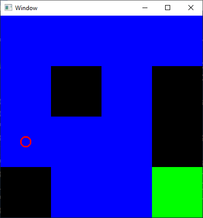
The last step is rendering the environment with a draw function. This just requires a working knowledge of constructing the Picture type in Gloss. It's a little tedious, so I won't belabor the details. Check the Github links at the bottom if you're curious!
We can then combine all these pieces like so:
main :: IO ()
main = do
  env <- basicEnv
  play windowDisplay white 20
    (World env GameInProgress)
    drawEnvironment
    handleInputs
    updateWorldTime
After we have all these pieces, we can run our game, moving our player around to reach the green tile while avoiding the black tiles!
CONCLUSION
With a little more plumbing, it would be possible to combine this with the rest of our "Environment" work. There are some definite challenges. Our current environment setup doesn't have a "time update" function. Combining machine learning with Gloss rendering would also be interesting.
This is the end of the Open AI Gym series, but take a look at our Github repository to see all the code we wrote in this series! The code for this article is on the gloss branch, particularly in FrozenLakeGloss.hs, with some modifications to FrozenLakeBasic.hs. If you liked this series, don't forget to Subscribe to Monday Morning Haskell to get our monthly newsletter!